
Fat-Tailed Models for Risk Estimation
Assistant Professor of Statistics and Econometrics,
![]() zye
zye![]() in University, Turkey
in University, Turkey
Risk models are employed in financial modeling to provide a measure of risk that could be employed in portfolio construction, risk management, and derivatives pricing. A risk model is typically a combination of a probability distribution model and a risk measure. In this entry, we discuss alternatives for building the probability distribution model, as well as the pros and cons of various heavy-tailed distributional choices. Our focus is univariate models; their multivariate extensions are only briefly mentioned. We start with the fundamentals—the Gaussian distribution. Then, we introduce fat-tailed alternatives, such as the Student’s t distribution and its asymmetric version and the Pareto stable class of distributions and their tempered extensions. Next, we discuss extreme value theory’s risk modeling approach. We conclude with a comparative empirical example to contrast the models’ performance over a 10-year period.
THE FUNDAMENTALS: NORMAL DISTRIBUTION
The use of normal (Gaussian) distribution in financial modeling has a long and distinguished tradition. The main reasons for its traditional popularity are several. First, its analytical tractability means that deriving theoretical results and employing it in applications is (relatively) straightforward; numerical methods are widely available and implementable.1 Second, certain central results in statistics underlie the importance of the Gaussian distribution.2 Third, it has an intuitive appeal—random variables distributed with the Gaussian distribution tend to assume values around the average, with the odds of deviation from the average decreasing exponentially as one moves away from it.
Some of the most prominent financial frameworks built around the normal distribution are Markowitz’s modern portfolio theory, the capital asset pricing model, and the Black-Scholes option pricing model. All of them assume (or imply) that asset returns follow a normal distribution and reflect a long-standing paradigm that rational investors’ preferences can be described exclusively in terms of expected returns and risk as measured by the variance of the return distribution. However, they are inherently static frameworks. The underlying dynamic is either given exogenously or is based on the assumption that returns have independent and identical distributions. Such characteristics do not fit adequately with the empirically observed features of financial returns and investor choice.
In this section, we describe the fundamentals of a risk modeling approach based on the Gaussian distribution. We start with a review of some of its basic properties and facts.
Basics and Properties of the Gaussian Distribution
The normal distribution is characterized by two parameters—a location (mean) parameter and a scale (volatility, standard deviation) parameter.3 The location parameter serves to displace (shift) the whole distribution, while the scale parameter changes the shape of the distribution. For small values of the scale, the distribution is narrow and peaked, while for (relatively) larger values, it widens and flattens. Since the normal distribution is symmetric around its mean, the location (mean) coincides with the center of the distribution. Commonly, the mean is denoted by μ and the standard deviation by σ.
Two important properties of the normal distribution are location-scale invariance and summation stability. They are directly related to the central role of the normal distribution in traditional financial modeling.
Location-Scale Invariance Property
Let us suppose a random variable X is normally distributed with parameters μ and σ. Now consider another random variable, Y, obtained as a linear function of X, that is, Y = aX+b. The variable Y is also normally distributed with parameters μ Y = aμ +b and σ Y = aσ. That is, if a normal random variable is multiplied by a constant and/or is shifted, it remains distributed with the normal distribution.
Summation Stability Property
Let us take n independent random variables distributed with the Gaussian distribution with parameters μ i and σ i. The sum of the variables is normal as well. The resulting normal distribution has a mean and standard deviation obtained, respectively, as
Location-scale invariance and summation stability are not universal properties of statistical distributions. In financial applications, however, they are clearly desirable properties.
The property of summation stability is often used to justify the predominant use of normal distributions in financial modeling. A statistical result, called the central limit theorem, states that, under certain technical conditions, the sum of a large number of random variables behaves like a normally distributed random variable. More generally, we say that the normal distribution possesses a domain of attraction. In fact, the normal distribution is not the only distribution with this feature. As we will see later in the entry, it is the class of stable distributions (to which the Gaussian distribution belongs) that is unique with that property. A large sum of random variables can only converge to a stable distribution.
Density Function and Fitting of the Normal Distribution
The density function of a random variable X distributed with the normal distribution with mean μ and standard deviation σ is given by the following expression
(1) ![]()
We denote this distribution as N(μ, σ). The variable X and the parameter μ can take any real value, while σ can only take positive values. A normal random variable with zero mean and standard deviation of one is said to be distributed with the standard normal distribution (N(0, 1)). The presence of the exponential function in the normal density implies that the probability of events away from the mean decays at an exponential rate. In contrast, heavy-tailed distributions are characterized by power-law behaviors for large (small) values of the random variables, leading to increased chance for extreme events relative to the Gaussian setting.
Fitting of the Gaussian distribution is usually performed by maximizing the logarithm of the likelihood function given by
(2) 
where x1, x2, …, xn is the sample of observed data used for fitting. The resulting estimators of the mean and the standard deviation are (using standard notation):
(3) ![]()
(4) ![]()
Unconditional models imply that returns are independent and identically distributed (IID), so that (among other implications) the returns’ means and variances remain unchanged through time. However, empirical evidence abounds that financial returns exhibit time-series properties such as autocorrelation and volatility clustering, which make unconditional return modeling inadequate. The time-series properties of returns need to be modeled in a conditional framework with appropriate time series models. We consider conditional normal models next.
Conditional Normal Models and Time-Series Properties of Returns
Properly computing the risk of a portfolio depends on recognizing a number of essential features of the evolution of returns through time. We begin with the two most commonly accounted for by academics and practitioners—autocorrelation and volatility clustering.
Sometimes, a portfolio’s past performance influences future performance. Current returns of a financial asset may depend on its past returns. This property of autocorrelation is modeled by including lagged (past) values of the return and/or lagged innovations (informational surprises). The resulting conditional model of the expected return is called an autoregressive moving average (ARMA) model.
Time-varying volatility concerns the empirically observed fact that large returns (of either sign) tend to be followed by large ones and small returns by small ones. To describe this volatility clustering effect, the class of autoregressive conditional heteroskedasticity (ARCH) models, as well as their generalized (GARCH) extensions are widely used. GARCH models assume that volatility on a given day depends on the volatilities and also squared innovations of the one or more previous days.
The typical approach to building a risk model includes at least the elements of autoregressive component and volatility clustering component by means of a GARCH or alternative ARCH-type processes. A conditional normal ARMA(1,1)-GARCH(1,1) model combines the returns’ conditional mean and volatility models with the assumption that returns are distributed with the Gaussian distribution. Analytically, the model is represented as
(5) ![]()
(6) ![]()
(7) ![]()
where rt, μ t, and σ 2t are the return, expected return, and return variance at time t, respectively, and ![]() is the innovation at time t. The innovation is normally distributed with mean 0 and variance σ 2t.4
is the innovation at time t. The innovation is normally distributed with mean 0 and variance σ 2t.4
The standardized fitted residuals, ![]() , are the original returns with the effects of autocorrelation and volatility clustering removed (filtered out). Since the model innovations are assumed to be Gaussian, if the model is correctly specified, these filtered returns must exhibit the dynamics of a Gaussian white noise with variance one. Therefore, one easy way to determine whether the distributional assumptions are valid is to examine the properties of these residuals. Indeed, numerous studies have confirmed that in the case of financial returns the standardized fitted residuals are not Gaussian. That is, even after removing the autocorrelation and volatility clustering, fat tails, though smaller in magnitude, continue to be present in returns. Time-varying volatility then is not sufficient to explain the extreme events observable in returns.5 Therefore, a more realistic risk model should allow for fat-tailed innovations. In the next section, we discuss parametric fat-tailed models, specifically, models based on the classical Student’s t distribution and its asymmetric version, as well as on the stable and tempered stable distributions.
, are the original returns with the effects of autocorrelation and volatility clustering removed (filtered out). Since the model innovations are assumed to be Gaussian, if the model is correctly specified, these filtered returns must exhibit the dynamics of a Gaussian white noise with variance one. Therefore, one easy way to determine whether the distributional assumptions are valid is to examine the properties of these residuals. Indeed, numerous studies have confirmed that in the case of financial returns the standardized fitted residuals are not Gaussian. That is, even after removing the autocorrelation and volatility clustering, fat tails, though smaller in magnitude, continue to be present in returns. Time-varying volatility then is not sufficient to explain the extreme events observable in returns.5 Therefore, a more realistic risk model should allow for fat-tailed innovations. In the next section, we discuss parametric fat-tailed models, specifically, models based on the classical Student’s t distribution and its asymmetric version, as well as on the stable and tempered stable distributions.
INCORPORATING HEAVY TAILS AND SKEWNESS: PARAMETRIC FAT-TAILED MODELS
The Student’s t distribution has become the “go to” mainstream alternative of the normal distribution, when attempting to address asset returns’ heavy-tailedness. Further below, we introduce an extension, called the skewed Student’s t distribution, designed to deal with data asymmetries. First, we turn to discussing the “classical” Student’s t distribution.
The “Classical” Student’s t Distribution
The Student’s t distribution (or simply the t-distribution) is symmetric and mound-shaped, like the normal distribution. However, it is more peaked around the center and has fatter tails. This makes it better suited for return modeling than the Gaussian distribution. Additionally, numerical methods for the t-distribution are widely available and easy to implement.
The t-distribution has a single parameter, called degrees of freedom (DOF), that controls the heaviness of the tails and, therefore, the likelihood for extreme returns. The DOF takes only positive values, with lower values signifying heavier tails. Values less than 2 imply infinite variance, while values less than 1 imply infinite mean. The t-distribution becomes arbitrarily close to the normal distribution as DOF increases above 30.
Density Function of the Student’s t Distribution
A random variable X (taking any real value) distributed with the Student’s t distribution with ![]() degrees of freedom has a density function given by
degrees of freedom has a density function given by
where “![]() ” is the Gamma function. We denote this distribution by
” is the Gamma function. We denote this distribution by ![]() . The mean of X is zero and its variance is given by
. The mean of X is zero and its variance is given by
(9) ![]()
The variance exists for values o
f ![]() greater than two and the mean—for
greater than two and the mean—for ![]() greater than one.
greater than one.
The t-distribution above is sometimes referred to as the “standard” Student’s t distribution.6 In financial applications, it is often necessary to define the Student’s t distribution in a more general manner so that we allow for the mean (location) and scale to be different from zero and one, respectively. The density function of such a “scaled” Student’s t distribution is described by
(10) 
where the mean μ can take any real value and σ is positive. The variance of X is then equal to ![]() . We denote the distribution above by
. We denote the distribution above by ![]() .7
.7
Finally, we make a note of an equivalent representation of the Student’s t distribution which is useful for obtaining simulations from it. The ![]() distribution is equivalently expressed as a scale mixture of the normal distribution where the mixing variable distributed with the inverse-gamma distribution,
distribution is equivalently expressed as a scale mixture of the normal distribution where the mixing variable distributed with the inverse-gamma distribution,
Later in this entry we will again come across mixture representations in the context of our discussion of the skewed Student’s t, the stable Paretian, and the classical tempered stable distributions.
Degrees of Freedom Across Assets and Time
The typical approach to risk modeling based on the Student’s t distribution includes building an autoregressive and volatility clustering components, as well as assuming that DOF is the same for all assets’ returns. This assumption is essential if we want to extend the classical Student’s t model to a multivariate one. It is, however, an empirical fact that assets are not homogeneous with respect to the degree of non-normality of their returns. Moreover, tail thickness and shape are not constant through time either.
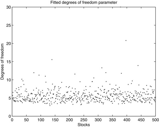
Consider the result of an empirical study of constituent stocks of the S&P 500 stock index during the period from January 2, 1991 to June 30, 2011. We calibrate the Student’s t distribution after filtering the equity returns for GARCH effects. The estimated DOF is shown in Figure 1. It is evident that tail behavior diverges dramatically across stocks. Around 44% of equity returns are very heavy tailed, with DOF estimate below five. Around 54% of equities have an estimated DOF parameter between five and 10. Only three stocks exhibit characteristics closer to the Gaussian, with a DOF exceeding 15. Obtaining accurate DOF estimates across assets is important in risk management, since these estimates can form the basis of an analysis of portfolio risk contributors and diversifiers.
Figure 1 Fitted Degrees-of-Freedom Parameter for S&P 500 Index Stock Returns
Note: The Student’s t distribution is calibrated on the residuals from a GARCH model fitted to the returns of the stocks in the S&P 500 index.
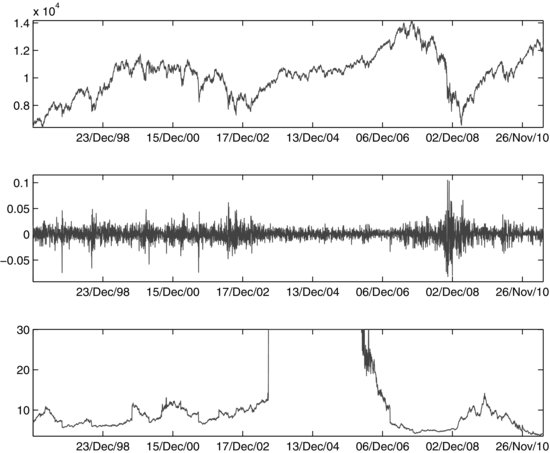
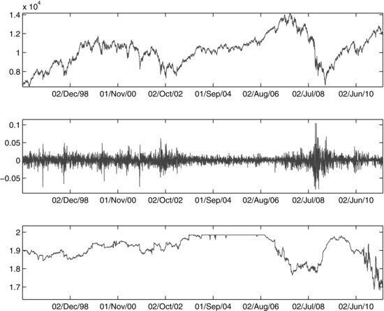
Not only does tail behavior vary across assets, it also changes through time. In relatively calm periods, asset returns are almost Gaussian, while in turbulent periods, the tails become fatter. Figure 2 illustrates the time-varying behavior of DOF, suggesting temporal tail dynamics for the Dow Jones Industrial Average (DJIA) returns for the period from January 1, 1997 to June 30, 2011. The top and middle plots show the value and return of the DJIA, respectively. The bottom plot shows the DOF parameter estimates.8 In periods of “normal” market volatility, returns are almost normally distributed, with a fitted DOF over 30. However, when markets are unsettled, return tails grow heavier. Accounting for that time dynamics is important in risk budgeting and management to serve as an indictor for the transition between different market regimes—from calm to turbulent market or vice versa.
Figure 2 Fitted Degrees-of-Freedom Parameter for DJIA Returns
Note: The Student’s t distribution is calibrated on the residuals from a GARCH model fitted to the return on the DJIA using a 500-day rolling window
As pointed out earlier, a major limitation of employing the classical Student’s t distribution for risk modeling is its symmetry. If there is significant asymmetry in the data, it will not be reflected in the risk estimate. There are at least several versions of the skewed Student’s t distribution, depending on the analytical way in which asymmetry is introduced into the distribution.9 Below, we consider the skewed Student’s t distribution obtained as a mixture of Gaussian and inverse-gamma distributions.10
The Skewed Student’s t Distribution
Suppose that a random variable X is distributed with the skewed Student’s t distribution, obtained as a mixture of a Gaussian distribution and an inverse-gamma distribution,
(11) ![]()
where
- W is an inverse-gamma random variable with parameters
 ,
,  .
. - Z is a Gaussian random variable,
 , independent of W.
The parameters μ and γ are real-valued. The sign and magnitude of γ control the asymmetry in X. We say that X’s distribution is a mean-variance mixture of the normal distribution, since the mixing variable W modifies both the mean and the variance of the Gaussian Z. Notice that conditional on the value of W, the distribution of X is normal:
(12) ![]()
X’s unconditional distribution is what is defined as the skewed Student’s t distribution and its density is given by the expression
where
and ![]() is the so-called modified Bessel function with index
is the so-called modified Bessel function with index ![]() .
.
Fitting and Simulation of the Classical and Skewed Student’s t Distributions
Estimation of the classical and skewed Student’s t distributions is carried out using the method of maximum likelihood. Simulations from the two distributions make use of their normal mixture representations. For given parameters μ, σ, and γ (e.g., the maximum likelihood estimates), generation of t and skewed t observations consists of the steps below:
- Generate an observation w from the inverse-gamma distribution with parameters
 .
. - Generate an observation z from the normal distribution with mean 0 and variance σ 2.
- Compute the corresponding observation of the t or skewed t-distribution, respectively, as
(13)

Stable Paretian and Classical Tempered Stable Distributions
Research on stable distributions in the field of finance has a long history.11 In 1963, the mathematician Benoit Mandelbrot first used the stable distribution to model empirical distributions that have skewness and fat tails. The practical implementation of stable distributions to risk modeling, however, has only recently been developed. Reasons for the late penetration are the complexity of the associated algorithms for fitting and simulating stable models, as well as the multivariate extensions. To distinguish between Gaussian and non-Gaussian stable distributions, the latter are commonly referred to as stable Paretian, Lévy stable, or α-stable distributions.
Stable Paretian tails decay more slowly than the tails of the normal distribution and therefore better describe the extreme events present in the data. Like the Student’s t distribution, stable Paretian distributions have a parameter responsible for the tail behavior, called tail index or index of stability.
Definition of Stable Paretian Distributions
We offer two definitions of the stable Paretian distribution. The first one establishes the stable distribution as having a domain of attraction. That is, (properly normalized) sums of IID random variables are distributed with the α-stable distribution as the number of summands n goes to infinity. Formally, let Y1, Y2, … , Yn be IID random variables and ![]() and
and ![]() be sequences of real and positive numbers, respectively. A variable X is said to have the stable Paretian distribution if
be sequences of real and positive numbers, respectively. A variable X is said to have the stable Paretian distribution if
(14) ![]()
where the symbol ![]() denotes convergence in distribution.
denotes convergence in distribution.
The density function of the stable Paretian distribution is not available in a closed-form expression in the general case. Therefore, the distribution of a stable random variable X is alternatively defined through its characteristic function. The density function can be obtained through a numerical method, as we explain further below. The characteristic function of the α-stable distribution is given by
(15) 
where ![]() is 1 if t>0, 0 if t = 0, and −1 if t<0. The four parameters uniquely determining the α-stable distribution are:
is 1 if t>0, 0 if t = 0, and −1 if t<0. The four parameters uniquely determining the α-stable distribution are:
- α: index of stability or tail index,
 .
. - β: skewness parameter,
 .
. - σ: scale parameter, σ >0.
- μ: location parameter,
 .
.
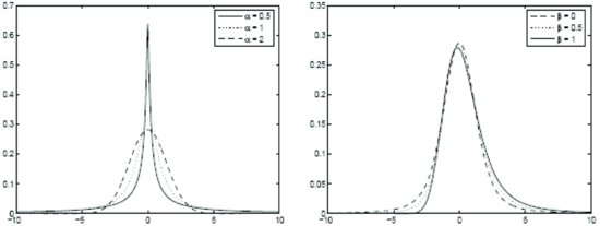
We denote the distribution by Sα(σ, β, μ). The roles of α and β are illustrated in Figure 3. The sign of β reflects the asymmetry of the distribution. Positive (negative) β implies skewness to the right (left). As noted earlier, the index of stability controls the degree of heavy-tailedness of the distribution. Smaller values imply a fatter tail. The closer the tail index is to two, the more Gaussian-like the distribution is. Indeed, for α = 2, we arrive at the Gaussian distribution—if X is distributed with S2(σ, β, μ), then it has the normal distribution with mean equal to μ and variance equal to 2σ 2. In this case, the parameter β loses its meaning as a skewness parameter and becomes irrelevant. Nevertheless, the normal distribution is usually associated with β = 0. Apart from the Gaussian distribution, there are two more special cases for which the density function of the stable distribution is available in a closed form: the Cauchy distribution (α = 1, β = 0) and the completely skewed Lévy distribution (α = 1/2, ![]() ).
).
Figure 3 Stable Density: μ = 0, σ = 1, β = 0, and varying α (left); α = 1.5, μ = 0, σ = 1, and varying β (right)
Basic Properties of the Stable Distribution
We outline three basic properties of the α-stable distribution:
- Power-tail decay. The tail of the stable distribution’s density decays like a power function (slower than the exponential decay). It is this property that allows the stable distribution to capture the occurrence of extreme events. For a constant C, the property can be expressed as
(16)

- Existence of raw moments. The magnitude of the tail index determines the order up to which raw moments exist:
(17)
This property implies that, for non-Gaussian α-stable distributions (α <2), the variance (as well as higher moments such as skewness and kurtosis) does not exist. When the index of stability has a value less than one, the mean is infinite as well. Since the variance does not exist, one cannot express risk in terms of the variance. However, the scale parameter can play the role of a risk measure, in the same way that the standard deviation does in the normal distribution case.
- Stability. The property of stability characterizes the preservation of the distributional form under linear transformations. It is governed by the index of stability α and expressed as follows. Suppose that X1, X2, … , Xn are IID random variables, independent copies of a random variable X. Then, for a positive constant Cn and a real number Dn, X follows the stable distribution:
(18)
The notation
 denotes equality in distribution. The constant Cn = n1/α determines the stability property. The stability property means that the “classical” central limit theorem does not apply in the non-Gaussian case. A large sum of appropriately standardized IID random variables is distributed with the stable Paretian distribution as the number of terms increases indefinitely, not with the normal distribution.
When the variables Xi, i = 1, … , n, are themselves distributed with the α-stable distribution, , the stability property can be extended further:
1. The distribution of
, the stability property can be extended further:
1. The distribution of is α-stable with index of stability α and parameters:
(19)
 2. The distribution of Y = X1+a for some real constant a is α-stable with index of stability α and parameters:
(20)
 3. The distribution of Y = aX1 for some real constant a (
 ) is α-stable with index of stability α and parameters:
Figure 4 Fitted Stable Tail Index for DJIA Returns
Note: The Stable Paretian distribution is calibrated on the residuals from a GARCH model fitted to the return on the DJIA using a 500-day rolling window
In empirical analysis, the time-varying tail behavior of assets is reflected in the nonconstancy of the tail index of the α-stable distribution, as demonstrated in Figure 4. As in the earlier illustration, the tail index is estimated by fitting a stable distribution to the filtered returns (after removing the volatility clustering with a GARCH model.) The tail index of the DJIA returns is very close to two in the upward market environment from 2003 to 2005 but starts decreasing right before the 2008 market crash and is smallest at the time of the crash itself. This implies that tail thickness is smallest in the bullish market from 2003 to 2005 and is largest during the crisis period.
As noted above, the variance of non-Gaussian stable distributions does not exist. To address this potentially undesirable feature, smoothly truncated stable distributions and various types of tempered stable distributions have been proposed. They are all obtained with a procedure known as “tempering” applied to the tails of the distribution to ensure that the variance is finite. This procedure replaces the power decay very far out in the tails of the distribution with an exponential (or faster) decay. We discuss the classical tempered stable distributions next.
Definition of Classical Tempered Stable Distributions
The characteristic function of the classical tempered stable (CTS) distribution is given by the following expression:
(21) ![]()
We denote the distribution by CTS(α, C, ![]() ,
, ![]() , m). The distribution parameters are characterized as follows:
, m). The distribution parameters are characterized as follows:
- α: tail index,
 .
. - m: location parameter,
 .
. - C: scale parameter, C>0.
 and
and  : parameters controlling the decay in the right and left tail, respectively;
  .
.
The relative magnitudes of ![]() and
and ![]() determine the degree of skewness of the CTS distribution. When
determine the degree of skewness of the CTS distribution. When ![]() (
(![]() ), the distribution is skewed to the left (right). Symmetry is obtained for
), the distribution is skewed to the left (right). Symmetry is obtained for ![]() . Tail heaviness is determined in a more flexible manner in the CTS distribution than in the stable Paretian distribution. Three parameters play a role in that:
. Tail heaviness is determined in a more flexible manner in the CTS distribution than in the stable Paretian distribution. Three parameters play a role in that: ![]() ,
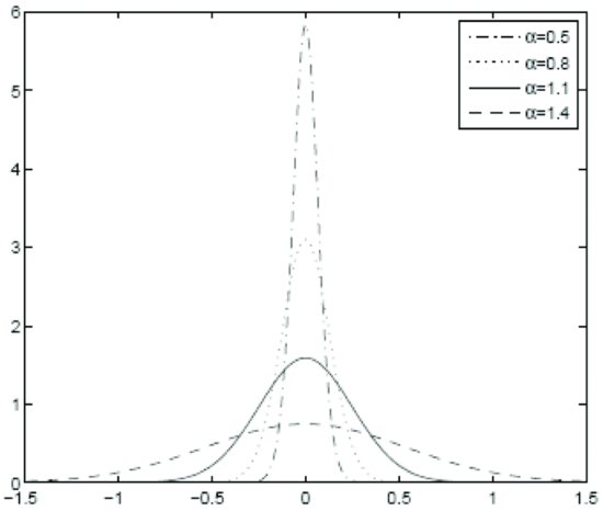
, ![]() , and α. The former two have the effect of scaling the tails (smaller values correspond to heavier tails), while the latter one, of shaping the tails (as before, small values imply fatter tails). The effect of different values of these three parameters on the CTS distribution can be seen in Figures 5, 6, and 7.
, and α. The former two have the effect of scaling the tails (smaller values correspond to heavier tails), while the latter one, of shaping the tails (as before, small values imply fatter tails). The effect of different values of these three parameters on the CTS distribution can be seen in Figures 5, 6, and 7.
Figure 5 Probability Density of the CTS Distribution: Dependence on ![]() and
and ![]()
Note: CTS Parameter Values: α = 0.8, C = 1, m = 0, and varying ![]() and
and ![]()
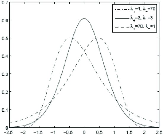
Figure 6 Probability Density of the Symmetric CTS Distribution: Dependence on ![]() and
and ![]()
Note: CTS Parameter Values: α = 1.1, C = 1, m = 0, and varying ![]() and
and ![]()

Figure 7 Probability Density of the CTS Distribution: Dependence on α
Note: CTS Parameter Values: C = 1, ![]() ,
, ![]() , m = 0, and varying α
, m = 0, and varying α
Linear combinations of CTS-distributed random variables are also distributed with the CTS distribution. First, we define the standard CTS distribution. A random variable X has the standard CTS distribution if
(22) ![]()
The distribution is denoted by ![]() . Its mean and variance are zero and one, respectively.
. Its mean and variance are zero and one, respectively.
For a positive number σ and a real number m, the linear combination Y = σ X+m has the CTS distribution:
(23) ![]()
The mean and variance of Y are m and σ 2, respectively.
Subordinated Representation of the α-Stable and CTS Distributions
Similar to the Student’s t distribution, stable distributions can be represented as mixtures of other distributions. More generally, (continuous) mixture representations are analyzed within the framework of intrinsic time change and subordination. The price and return dynamics can be considered under two different time scales—the physical (calendar) time and an intrinsic (also called operational, trading or market) time. The intrinsic time is best thought of as the cumulative trading volume process which measures the cumulative trading volume of the transactions up to a point on the calendar-time scale. It is a measure of market activity and a reflection of the empirical observation that price changes are larger when market activity is more intense. Let us denote the intrinsic time process by T(t) and the time-evolving random variable such as price or return by X(t). X(t) is assumed independent of T(t). The compound process X(T(t)) is said to be subordinated to X by the intrinsic time T(t) and T(t) is referred to as a subordinator.12 Since the increments of the intrinsic time ![]() are non-decreasing and positive, distributions such as gamma, Poisson, and inverse-Gaussian can be used to describe them in probabilistic terms.13 Another distributional alternative is the completely skewed to the right α-stable distribution, Sα(σ, 1, 0), for 0<α <1, whose support is the positive real line. Therefore, when 0<α <2, the subordinator is a stable distribution given by
are non-decreasing and positive, distributions such as gamma, Poisson, and inverse-Gaussian can be used to describe them in probabilistic terms.13 Another distributional alternative is the completely skewed to the right α-stable distribution, Sα(σ, 1, 0), for 0<α <1, whose support is the positive real line. Therefore, when 0<α <2, the subordinator is a stable distribution given by ![]() .
.
Subordinated models with random intrinsic time, such as X(T(t)), are leptokurtic. They have heavier tails and higher peaks around the mode of zero than the normal distribution. As such, they provide a natural way to model the tail effects observed in prices and returns.
Subordinated representations’ usefulness is in allowing for practical ways of simulating random numbers from the corresponding models. Subordinated processes are especially important in multiasset settings, where each marginal distribution has a different tail heaviness. This across-asset heterogeneity can be modeled by having subordinators with different parameters for each asset. As noted earlier, this characteristic of multivariate asset returns is crucially important for a realistic risk model able to identify tail risk contributors and tail risk diversifiers.
The subordinated representation of the α-stable distribution can be expressed in the following way. Let Z be a standard normal random variable, ![]() , and Y be a positive α /2-stable random variable independent of Z,
, and Y be a positive α /2-stable random variable independent of Z, ![]() , where
, where
(24) ![]()
Then, the variable
![]()
is symmetric α-stable: ![]() . This implies that every symmetric stable variable is conditionally Gaussian (conditional on the value of the stable subordinator). Unconditionally, the symmetric α-stable distribution is expressed as a scale mixture of normal distributions.14
. This implies that every symmetric stable variable is conditionally Gaussian (conditional on the value of the stable subordinator). Unconditionally, the symmetric α-stable distribution is expressed as a scale mixture of normal distributions.14
The CTS distribution has a subordinated representation as well and can be expressed as a mean-scale mixture of Gaussian distributions. For details, see Madan and Yor (2005).
Fitting and Simulations of α-Stable and CTS Distributions
Fitting techniques for the α-stable distributions can be divided into three categories: quantile methods, characteristic function-based methods, and maximum likelihood methods. The quantile method is similar to the method of moments estimation method in that it uses predetermined empirical quantiles to estimate the sample parameters.15 The characteristic function-based methods also resemble the method of moments and rely on transformations of the sample characteristic function.16 Finally, the latter method involves maximization of the likelihood function, which is computed numerically. Comparative studies of the three fitting approaches show that the method of maximum likelihood is superior in terms of estimation accuracy. The quantile method requires the least amount of computational time but is the least accurate one. The second category of methods also have the benefit of computational simplicity but may have a difficulty in estimating the skewness parameter.17 For these reasons, here we focus on the method of maximum likelihood in some more detail.
In statistical theory, the relationship between the probability density function (pdf) and the characteristic function is expressed as follows:
where h>0 and ![]() and
and ![]() are the density and characteristic functions, respectively. The pdf of the α-stable and CTS distributions can be computed by numerical evaluation of the integral above. A fast and computationally efficient method of numerical integration is the fast Fourier transform (FFT) algorithm.18 Consider the pdf computation in (25). The main idea of FFT is to evaluate the integral for a grid of equally-spaced values of the random variable X:
are the density and characteristic functions, respectively. The pdf of the α-stable and CTS distributions can be computed by numerical evaluation of the integral above. A fast and computationally efficient method of numerical integration is the fast Fourier transform (FFT) algorithm.18 Consider the pdf computation in (25). The main idea of FFT is to evaluate the integral for a grid of equally-spaced values of the random variable X:
(26) ![]()
That is, equation (25) can be expressed as
This integral can be approximated by the so-called Riemann sum, after choosing small enough lower and large enough upper bounds:
(27) 
for k = 1, … , N. Here, the lower and upper bounds equal ![]() and
and ![]() , respectively. The distance between the grid points
, respectively. The distance between the grid points ![]() , n = 1, … , N is s. If
, n = 1, … , N is s. If ![]() , we arrive at the following expression for the density, after some algebraic rearrangement:
, we arrive at the following expression for the density, after some algebraic rearrangement:
(28) 
To compute the sum above, one can use the FFT implemented by many numerical analysis software packages. The parameters of the FFT method are N, the number of summands in the Riemann sum, and h, the grid spacing. Their values can be chosen appropriately, so as to achieve a balance between approximation accuracy and computational burden.19 Finally, the maximum-likelihood estimates of the parameters of the α-stable and CTS distributions are obtained by numerical maximization of the log-likelihood function.
Simulations of α-stable distribution can be accomplished using an algorithm called the Chambers-Mallows-Stuck generator. To generate a random number from Sα(σ, β, μ), the steps are as follows:
- Generate two independent random numbers from an exponential distribution with mean 1,
 , and from a uniform distribution,
  .
. - If
 , compute
(29)

where
(30)
- If α = 1, compute
(31)
- The random variable Z has a standardized stable distribution with location parameter equal to zero and scale parameter equal to one,
 . To obtain an observation from Sα(σ, β, μ) with arbitrary values of σ and μ, transform Z according to20
(32)

Conditional Parametric Fat-Tailed Models
A fat-tailed parametric model includes the following main components:
- An autoregressive component to capture autoregressive behavior.
- A volatility clustering component, usually a GARCH-type model.
- A fat-tailed distribution (stable Paretian or skewed Student’s t) to explain the heavy tails and the skewness of the residuals from the ARMA-GARCH model.
- Tail thickness changing with time and across assets addressed.
INCORPORATING HEAVY TAILS AND SKEWNESS: SEMI-PARAMETRIC FAT-TAILED MODELS
In this section, we review semi-parametric models, which combine an empirical distribution for the body of the data distribution where plenty of observations are available and extend the tail by a parametric model based on extreme value theory (EVT). EVT has a long history of applications in modeling the occurrence of severe weather, earthquakes, and other extreme natural phenomena. In general terms, extreme value distributions are the asymptotic distributions for the normalized largest observations of IID random variables. There are two main categories of models for extreme values: block maxima models and threshold exceedances models.
In the financial applications context, block maxima could refer to the maximal observations within certain predefined periods of time. For example, daily return data could be divided into quarterly (or semiannual or yearly) blocks and the largest daily observations within these blocks collected and analyzed. The distribution of the maximal values is generally not known. However, when the block size is large, so that block maxima are independent (irrespective of whether the underlying data are dependent), the limit distribution is given by EVT.21 The number of blocks determines the size of the data sample available for analysis and fitting. In contrast, in threshold exceedances models, the sample size is not predetermined but, naturally, depends on the a priori selected threshold level.
The first model category is represented by the so-called generalized extreme value (GEV) distribution. Its distribution function has the form
(33) 
where ![]() . The parameters
. The parameters ![]() ,
, ![]() , and σ >0 are the shape, location, and scale parameters, respectively. The value of
, and σ >0 are the shape, location, and scale parameters, respectively. The value of ![]() determines the three distributions encompassed by the parametric form above: the Weibull distribution (
determines the three distributions encompassed by the parametric form above: the Weibull distribution (![]() ), the Gumbel distribution (
), the Gumbel distribution (![]() ), and the Fréchet distribution (
), and the Fréchet distribution (![]() ). Of the three, the latter one has the heaviest tails,22 while the first one is short-tailed, with a finite right endpoint and, thus, not favored in modeling financial losses.23
). Of the three, the latter one has the heaviest tails,22 while the first one is short-tailed, with a finite right endpoint and, thus, not favored in modeling financial losses.23
The block maxima method’s major drawback is its “wastefulness” of data: all but the largest observation within each block are discarded. For this reason, a more common approach to EVT modeling is the threshold exceedance method. In it, the extreme events exceeding a predetermined high level (that is, events in the tail) are modeled with the generalized Pareto distribution (GPD). Its distribution function is given by
(34) ![]()
where σ >0 and ![]() when
when ![]() and
and ![]() when
when ![]() . The parameters
. The parameters ![]() and σ are the shape and scale parameters, respectively. Like the GEV, the GPD contains several special cases defined by the value of
and σ are the shape and scale parameters, respectively. Like the GEV, the GPD contains several special cases defined by the value of ![]() . When
. When ![]() , we get the Pareto distribution with parameters
, we get the Pareto distribution with parameters ![]() and
and ![]() , whose tails exhibit slow, power-law decay. The exponential distribution is obtained for
, whose tails exhibit slow, power-law decay. The exponential distribution is obtained for ![]() ; its tails decay at an exponential rate. A short (finite)-tailed distribution, called Pareto type II distribution, arises when
; its tails decay at an exponential rate. A short (finite)-tailed distribution, called Pareto type II distribution, arises when ![]() . 24
. 24
Fitting and Simulations of the GPD
In empirical modeling, there is generally a perceived trade-off between fitting the bulk and the tails of the data. Data around the mode are numerous and relatively easy to fit, while data in the tails are sparse and present an estimation challenge. Most commonly, the choice of model is based on how well it fits the bulk of the data, with the tails relegated to a somewhat secondary role. The semiparametric approach we consider in this section is to describe the majority of the data in a nonparametric fashion and use the GPD to fit the tails. Since the GPD describes the excess distribution over a threshold, we now define formally this concept.
For a random variable with cumulative distribution function G, the excess distribution over the threshold u is denoted by Gu and is given by
for ![]() , where xF is the right endpoint (a finite number or infinity) of X’s distribution function G.25 A statistical result known as the Pickand-Balkema-de Haan theorem implies that the excess distributions of a large class of underlying distributions converge to a GPD as the threshold level increases. That is, GPD is the limiting distribution as u increases to infinity.
, where xF is the right endpoint (a finite number or infinity) of X’s distribution function G.25 A statistical result known as the Pickand-Balkema-de Haan theorem implies that the excess distributions of a large class of underlying distributions converge to a GPD as the threshold level increases. That is, GPD is the limiting distribution as u increases to infinity.
Denote the available data sample by X1, … , XN and define an upper and a lower threshold level uU and uL, respectively. The data points beyond the threshold levels constitute the tails of the data distribution that are to be modeled with EVT. Naturally, separate modeling of the two tails has the purpose of accounting for the potential skewness in the data distribution. Let us define the exceedances of uU by Yk,U = Xk−uU, where Xk>uU and the exceedances of uL by Yk,L = uL−Xk, where Xk<uL, k = 1, … , K.26 The estimates of the scale and shape parameters are most conveniently obtained by maximizing the GPD log-likelihood function for each of the sets of data Yk,U and Yk,L.27 It is written as
where ![]() denotes the GPD density function.
denotes the GPD density function.
The empirical distribution is usually estimated using kernel density estimation approach. The kernel density estimate can be roughly thought of as a smoothed-out histogram. A parameter, called bandwidth or window width, controls the degree of smoothness of the resulting density estimate. More formally, the kernel density estimate is defined as
where xi = (x1, x2, … , xn) is data sample coming from some unspecified distribution and assumed to be IID. The bandwidth, h, takes positive values and K is called the kernel, a symmetric function that integrates to one. The normal density is often chosen as the kernel in (36). The bandwidth’s value can be selected in an optimal way.28
The approach to scenario generation from a model based on GPD is also semiparametric—the body of the distribution is simulated from the empirical density and GPD tails are attached to it. Generating observations from a GPD with a given shape parameter ![]() , a scale parameter σ, and a threshold level u can be accomplished in the following three steps:
, a scale parameter σ, and a threshold level u can be accomplished in the following three steps:
- Generate an observation U from a uniform distribution on the interval (0, 1).
- Compute the quantity
(37)

- Compute the GPD realization as
(38)

Scenarios from the body of the distribution are generated nonparametrically, via historical simulation known as bootstrapping (or resampling, more generally). The procedure involves drawing randomly, with replacement, from the set of historically observed data points. The simulated tails of the distribution are then “attached” to the scenarios from the body to obtain semiparametric scenarios from the whole data distribution.
Threshold Selection
We consider two of the most popular tools for selection of the threshold level—the mean excess function plot and the Hill plot. Both of them rely on visual inspection to determine the threshold.
The mean excess function is closely related to the concept of excess distribution. It describes the average exceedance above a threshold u, as a function of u.29 Formally, it is defined as
(39) ![]()
In the case of the GPD, m(u) can be shown to equal
![]()
where ![]() if
if ![]() and
and ![]() if
if ![]() . The excess mean function does not exist for
. The excess mean function does not exist for ![]() . The mean excess function is linear in the threshold level. This linearity is used to motivate a graphical check that the data conform to a GPD model: If the plot is approximately linear for high threshold values, the GPD may be employed to describe the distribution of the exceedances. The level above which linearity is evident may be taken as the threshold level.
. The mean excess function is linear in the threshold level. This linearity is used to motivate a graphical check that the data conform to a GPD model: If the plot is approximately linear for high threshold values, the GPD may be employed to describe the distribution of the exceedances. The level above which linearity is evident may be taken as the threshold level.
Plots of the Hill estimator are another EVT model selection method. The Hill approach offers a way to estimate the tail index ![]() . Denote the ith order statistics of the data sample by X(i).30 The Hill estimator of α is defined as
. Denote the ith order statistics of the data sample by X(i).30 The Hill estimator of α is defined as
(40) 
where ![]() and m is a sufficiently high number. For
and m is a sufficiently high number. For ![]() , the Hill estimator is equal to α asymptotically, as the sample size n and the number of extremes m increase without bound. In practical applications, the Hill estimator is computed for different values of m and plotted against these values. The plot is expected to stabilize above a certain value of m, so that the Hill estimates constructed from a different number of order statistics remain approximately the same. The threshold level u is then estimated by X(m).
, the Hill estimator is equal to α asymptotically, as the sample size n and the number of extremes m increase without bound. In practical applications, the Hill estimator is computed for different values of m and plotted against these values. The plot is expected to stabilize above a certain value of m, so that the Hill estimates constructed from a different number of order statistics remain approximately the same. The threshold level u is then estimated by X(m).
The semiparametric approach described in this section is a source of two major challenges. First, in order to obtain a sufficiently large number of observations in the tail, a large sample of historical data is needed. Second, even though the plots of the Hill estimator and the mean excess function provide a method for threshold identification, such identification is intrinsically subjective, as it is based on visual inspection. Moreover, it is difficult to automate it for large-scale applications.31
Conditional GPD Approach
The semiparametric approach described above is unconditional, since it implicitly assumes that the observed data is IID. A typical conditional GPD approach involves the components:
- Autoregressive model to capture linear dependencies in the data.
- GARCH-type model to capture the volatility clustering in the data.
- Semi-parametric model applied to the standardized residuals (which are approximately IID) to explain the data’s heavy-tailedness and asymmetry.
COMPARISON AMONG RISK MODELS
Using the DJIA daily returns from February 7, 1992 to June 30, 2011, we conduct a backtesting analysis to compare the three fat-tailed distribution models—stable Paretian, Student’s t, and EVT—alongside the normal distribution model. The data used in all models are first filtered for autoregression and volatility clustering using ARMA-GARCH.
The particular models we use in this section are the univariate analogs of the typical approaches to modeling in the multivariate case. A short discussion will help clarify what this means. Earlier we explained that, in a multi-asset setting, taking into account the varying tail behavior of the returns of different assets is of principal importance for risk analysis and management. However, employing the classical Student’s t distribution in the multivariate case necessarily implies the same value of the DOF parameter for all assets. That value would “average out” the tail-fatness of assets, so that the risk of some risk drivers will be underestimated, while the risk of others, overestimated. To reflect this typical multivariate application, in our backtesting analysis we choose to fix the DOF of the Student’s t distribution to four.
In the case of the stable Paretian model, similar considerations about the heterogeneity of tail behavior across risk drivers lead us to use the subordinated representation of the α-stable distribution. As mentioned in an earlier section, that representation allows for modeling the individual tail behavior of assets.
The backtesting analysis in this section, therefore, can be understood as a comparison among models with increasing degree of sophistication. We start with the classical parametric approach (the “Gaussian model”). Then, a “non-sophisticated” fat-tailed model, represented by the fixed-DOF Student’s t model (the “T-model”) is tested. Finally, a state-of-the-art fat-tailed model—the stable subordinated model (the “stable model”)—is considered. For each of the four models, exceedances of value-at-risk (VaR)—the number of times the realized loss is larger than the predicted VaR level—are tracked.32 We run the backtest with the following settings:
- Backtest period: January 2, 2004, to June 30, 2011.
- VaR confidence level: 99%.
- Time window: 500 rolling days for normal, classical Student’s t, and stable Paretian distributions and 3,000 rolling days for EVT.33
- EVT threshold: 1.02% (as suggested by Goldberg, Miller, and Weinstein (2008)).
The number of exceedances of the daily 99% VaR in the backtesting analysis for the four models is summarized below:
| Model | Number of Exceedances |
| Stable | 21 |
| Student’s t | 26 |
| Gaussian (normal) | 42 |
| EVT | 1 |
The number of exceedances is compared using a 95% confidence interval estimated to be [10, 27]. The results show that the Gaussian model is too optimistic—with 42 exceedances, its VaR forecasts are too low. In contrast, the EVT approach is overly pessimistic: Its predicted VaR is only exceeded once in the backtesting period. The Student’s t model and the stable model both produce exceedances within the confidence interval, with the latter model being very close to the upper bound.
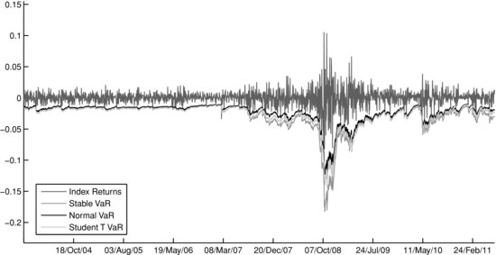
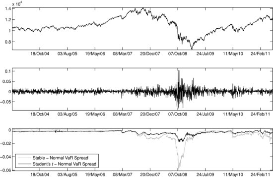
The DJIA performance during the backtest period is presented in Figure 8. Figure 9 plots the daily 99% VaR forecast produced by the Gaussian model, the Student’s t model, and the stable model against the daily DJIA returns for the full backtest period. Since the EVT model’s VaR predictions are too conservative, we have excluded it from the exhibit for the sake of presentation clarity. It can be seen from the figure that in times of low market volatility, the VaR forecasts of the three models are almost indistinguishable. However, during periods of greater market turmoil, differences in predicted risk levels are substantial across models. This point is further elaborated in Figure 10, which shows the spreads between the 99% VaR forecasts for the Student’s t Gaussian and the stable-Gaussian model pairs, along with the values and returns of DJIA. We observe that the stable-Gaussian VaR spread stays at zero for the period from 2004 to late-2006, suggesting “normal” market conditions. (The estimated tail index parameter of the α-stable distribution is close or equal to two during that period.) This is an essential feature of the stable model: Despite being a fat-tailed approach, it does not overpenalize the portfolio by assessing unnecessarily high risk estimates during calm market periods. On the other hand, even in times of severe market circumstances the number of exceedances of the stable VaR is within an acceptable range. For the period from June 1, 2008 to June 1, 2009, the stable VaR has one exceedance, which is within the 95% confidence interval for the number of exceedances ([0, 4]). By comparison, the Student’s t model’s VaR is exceeded four times, while the Gaussian model has seven exceedances.
Figure 8 Dow Jones Industrial Average Performance: January 2, 2004–June 30, 2011
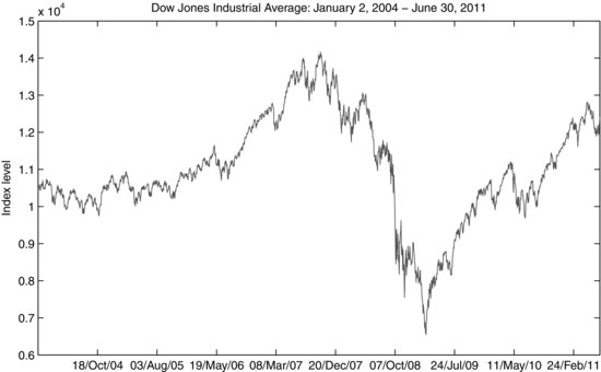
Figure 9 Backtest of the 99% Daily VaR Predicted by Different Distributional Methodologies
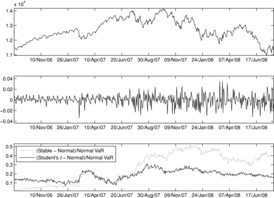
It is interesting to analyze whether the VaR forecasts can anticipate the transition from a calm market regime to a turbulent one. To investigate, we “zoom in” on the VaR spread dynamics for the two-year period leading up to the September 2008 crash. Figure 11 shows the VaR spreads for the period September 1, 2006–September 1, 2008, relative to the Gaussian VaR forecast. We notice that the stable-Gaussian relative spread starts increasing in
Figure 10 Spreads between 99%VaR Predictions for Student’s t Gaussian and Stable-Gaussian Model Pairs: Full Period
late 2006. This is the result of the increased tail-fatness estimated by the stable model (α decreases). At the same time, the Student’s t–Gaussian relative spread is fairly constant due to the fact that the DOF (and, therefore, the tail-fatness) is fixed.34 Over the two-year period, we can see a pronounced increase in the stable-Gaussian VaR relative spread. There are two time segments (in spring 2007 and spring 2008) in which the spread actually decreases. Both are associated with periods following major negative news and market tremors.35 In these periods, the Gaussian model’s VaR “catches up” post factum due to the increase in the estimates of the conditional GARCH volatility.
Figure 11 Relative Spreads between 99%VaR Predictions for Student’s t Gaussian and Stable-Gaussian Model Pairs: September 1, 2006–September 1, 2008
In general, one can interpret the upward trend of the stable-Gaussian VaR relative spread as an indicator of markets accumulating higher probability of extreme events before the actual market volatility goes up. This predictive behavior is only possible due to the time-varying estimates of the tail-fatness (the α parameter in the stable model). Thus, in the fixed-DOF Student’s t model, such a predictive trend cannot be observed. During the two-year period, the number of exceedances is eight for the stable model, ten for the Student’s t model, and 16 for the Gaussian model, while the 95% confidence interval is [0, 9].
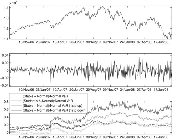
Finally, to test the significance of the stable-Gaussian VaR relative spread, we build a confidence interval for it. We do that by altering the tail index α at each point in time during the backtesting period with plus and minus one standard deviation of α and then recomputing the stable VaR and the associated stable-Gaussian relative spread. The standard deviation of α is estimated using parametric bootstrap, based on 200 bootstrap samples of 500 random draws each generated from an α-stable model with the corresponding α.36 Figure 12 shows the confidence bounds of the stable-Gaussian VaR relative spread for the two-year period running up to September 2008, together with the Student’s t–Gaussian VaR relative spread. Even the lower bound of the confidence interval of the stable-Gaussian VaR relative spread is more indicative than the Student’s t–Gaussian relative spread over this time period. Although the upward trend of the lower confidence bound is not as strong as that of the upper confidence bound, the results support the conclusion that the stable model’s VaR forecasts have the ability to anticipate a switch from a calm to a volatile market regime.
Figure 12 Relative Spreads between 99%VaR Predictions for Student’s t Gaussian and Stable-Gaussian Model Pairs with Confidence Bounds: September 1, 2006–September 1, 2008
KEY POINTS
- The Gaussian distribution is not adequate to describe the empirical features of asset returns. The standardized residuals from a conditional Gaussian model exhibit heavy-tailedness and asymmetry.
- The Student’s t distribution has fatter tails than the normal distribution. To account for skewness, however, the “classical” Student’s t distribution needs to be modified.
- The skewed Student’s t distribution can be represented as a mean-scale mixture of normal distributions; that is, normal distribution with random mean and variance.
- The tails of the stable Paretian distributions decay more slowly than the tails of the normal distribution and therefore better describe the extreme events present in the data.
- In the non-Gaussian case, a large sum of appropriately standardized IID random variables is distributed with the stable Paretian distribution in the limit.
- To address the issue of infinite variance, the stable Paretian distribution may be modified by tempering of the distribution’s tail. This gives rise to the tempered stable distributions.
- There are two main categories of distributions for extreme values—block maxima models and threshold exceedances models. The latter category is more often employed in risk modeling, since it is less “wasteful” of historical data than the former category.
- Selection of the threshold from where the tail of the data distribution starts is based on a subjective judgement and, together with data scarcity, is the main bottleneck in EVT applications.
- In all cases, before applying a fat-tailed model, an ARMA-GARCH filter should be used to remove the temporal dependence in asset returns.
- A realistic distributional assumption for a model should allow for tail-fatness that changes over time and from asset to asset. Such models can serve as early warning indicators when moving to a new market regime (from calm to turbulent and vice versa) and can identify tail-risk contributors and tail-risk diversifiers.
NOTES
1. The Gaussian distribution’s analytical tractability in the multivariate setting is an additional important factor behind its widespread use. See, for example, Kotz, Johnson, and Balakrishnan (2000) for details on the multivariate normal distribution.
2. However, later in this entry we provide an important clarification regarding a statistical result, called the central limit theorem.
3. In general, the scale parameter does not always coincide with the standard deviation (volatility), as we will see, for instance, in our discussion of the scaled Student’s t distribution later in the entry.
4. See, for example, Rachev, Stoyanov, Biglova, and Fabozzi (2005).
5. The conditional distribution of returns according to the model above is Gaussian. The unconditional distribution, however, is not normal but a mixture of normal distributions (due to the time-varying mean and variance). Its tails are fatter than those of the normal distribution but not fat enough to account for the empirically observed heavy tails.
6. Note that this is not the same as “standardized,” since the standard deviation of X is not one.
7. Notice that the Student’s t distribution defined in equation (8) has a location of zero and a scale of one.
8. More precisely, we estimate a GARCH model on a 500-day rolling window of returns and then fit a t-distribution to the (standardized) GARCH residuals.
9. Skewed Student’s t models have been proposed by Fernandez and Steel (1998), Azzalini and Capitanio (2003), and Rachev and Rüschendorf (1994), among others.
10. The skewed Student’s t distribution belongs to a more general class of distributions called generalized hyperbolic distributions and introduced by Barndorff-Nielsen (1978). It contains the Student’s t and normal distributions as limiting cases.
11. See Rachev and Mittnik (2000) and Samorodnitsky and Taqqu (1994). A detailed description of the stable methodology is available in Rachev, Martin, Racheva-Yotova, and Stoyanov (2009).
12. For details on the statistical properties of subordinated processes, see Feller (1966) and Clark (1973). Rachev and Mittnik (2000) provide discussions of subordinated processes in financial applications.
13. More generally, the family of infinitely divisible distributions to which the gamma, Poisson, inverse-Gaussian, and all stable Paretian distributions belong is a natural choice of distributions for the increments of the intrinsic time process T(t).
14. In a multivariate setting, Z would be distributed with a multivariate normal distribution and Y can be a a vector whose components are stable subordinators with different tail-fatness. The resulting distribution is a generalization of the multivariate sub-Gaussian stable distribution.
15. McCulloch (1986)’s estimation procedure generalized the quantile method for symmetric α-stable distributions of Fama and Roll (1971).
16. See Press (1972). Kogon and Williams (1998) and Koutrouvelis (1980) suggested regression-type estimator algorithms, also based on the characteristic function.
17. Comparison among the three types of estimation categories is provided in Stoyanov and Racheva-Yotova (2004).
18. A detailed description of the stable fitting methodology is available in Rachev and Mittnik (2000).
19. Rachev and Mittnik (2000) show that selecting h = 0.01 and N = 213 reduces the approximation error in computing the α-stable pdf to the satisfactory level of 10−6.
20. The algorithm for simulations from the CTS distribution is rather involved and described in detail in Rachev, Kim, Bianchi, and Fabozzi (2011).
21. The role of EVT in modeling maxima of random variables is similar to the one the central limit theorem plays in modeling the sums of random variables. Both characterize the limiting distributions.
22. The tails of the Fréchet distribution decay like a power function at a rate ![]() , the tail index parameter characterizing the α-stable distribution.
, the tail index parameter characterizing the α-stable distribution.
23. Comprehensive discussion of EVT is available in McNeil, Frey, and Embrechts (2005).
24. For more details on GPD, see Embrechts, Klüppelberg, and Mikosch (1997).
25. Notice that the threshold level u is in fact the location parameter in the GPD distribution.
26. The thresholds uL and uU are usually defined in terms of symmetric empirical quantiles, for example, the 5% and 95% quantiles. In that case, the number of observed data points in each tail is equal to K.
27. To be precise, when fitting the left tail, (35) is maximized over the absolute values of Yk,L, k = 1, … , K.
28. See, for example, Silverman (1986).
29. m(u) is also known as mean residual life function in survival analysis and characterizes the expected residual lifetime of a component that has function for u units of time already.
30. The ith order statistic is the ith largest observation in a data sample. The first order statistic is the maximum of the sample, while the nth order statistic is the minimum of a sample of size n.
31. See Rachev, Racheva-Yotova, and Stoyanov (2010) for a detailed discussion of these challenges.
32. Value-at-risk is defined as the minimum loss at a given confidence level for a predefined time horizon.
33. Goldberg, Miller, and Weinstein (2008) use time windows ranging from approximately 1,500 to 7,600 days.
34. The small variations are due to the variability in the estimates of the Student’s t GARCH model.
35. In February 2007, Freddie Mac announced that it would no longer buy the most risky subprime mortgages and mortgage-related securities and in April 2007, New Century Financial Corporation, a leading subprime mortgage lender, filed for Chapter 11 bankruptcy protection. Then, in the spring of 2008, we observed the collapse of Bear Stearns and the associated events.
36. The bootstrap sample size is 500, since this is the length of the time window used to calibrate the model.
REFERENCES
Azzalini, A., and Capitanio, A. (2003). Distributions generated by a perturbation of symmetry with emphasis on multivariate skew t-distribution. Journal of the Royal Statistical Society, Series B 65, 2: 367–389.
Barndorff-Nielsen, O. (1978). Hyperbolic distributions and distributions on hyperbolae. Scandinavian Journal of Statistics 5: 151–157.
Clark, P. (1973). A subordinated stochastic process model with finite variance for speculative prices. Econometrica 41, 1: 135–155.
Embrechts, P., Klüppelberg, C., and Mikosch, T. (1997). Modeling Extremal Events for Insurance and Finance. Springer.
Fama, E., and Roll, R. (1971). Parameter estimates for symmetric stable distributions. Journal of the American Statistical Association 66: 331–338.
Feller, W. (1966). An Introduction to Probability Theory and Its Applications. Hoboken, NJ: Wiley.
Fernandez, C., and Steel, M. (1998). On Bayesian modeling of fat tails and skewness. Journal of the American Statistical Association 93, 441: 359–371.
Goldberg, L., Miller, G., and Weinstein, J. (2008). Beyond value-at-risk: Forecasting portfolio loss at multiple horizons. Journal of Investment Management 6, 2: 73–98.
Hull, P., and Welsh, A. (1985). Adaptive estimates of parameters of regular variation. Annals of Statistics 122, 1: 331–341.
Kogon, S., and Williams, D. (1998). Characteristic function based estimation of stable parameters. In R. Adler, R. Feldman, and M. Taqqu (eds.), A Practical Guide to Heavy Tails, Birkhauser.
Kotz, S., Johnson, N. L., and Balakrishnan, N. (2000). Continuous Multivariate Distributions: Models and Applications. Hoboken, NJ: Wiley & Sons.
Koutrouvelis, I. (1980). Regression-type estimation of the parameters of stable laws. Journal of the American Statistical Association 7: 918–928.
Madan, D., and Yor, M. (2006). CGMY and Meixner Subordinators are Absolutely Continuous with Respect to One Sided Stable Subordinators. Cornell University Library, arXiv:math/0601173v2 [math.PR].
Mandelbrot, B. (1963). The variation of certain speculative prices. Journal of Business 26: 394–419.
McCulloch, J. (1986). Simple consistent estimators of stable distribution parameters. Communications in Statistics. Simulation and Computation 15: 1109–1136.
McNeil, A., Frey, R., and Embrechts, P. (2005). Quantitative Risk Management: Concepts, Techniques, and Tools. Princeton: Princeton University Press.
Press, S. (1972). Estimation in univariate and multivariate stable distribution. Journal of the American Statistical Association 67: 842–846.
Rachev, S., Kim, Y., Bianchi, M., and Fabozzi, F. (2011). Financial Models with Levy Processes and Volatility Clustering. Hoboken, NJ: Wiley.
Rachev, S., Martin, D., Racheva-Yotova, B., and Stoyanov, S. (2009). Stable ETL, optimal portfolios and extreme risk management, in G. Bol (ed.), Risk Assessment: Decisions in Banking and Finance, Physica, Springer.
Rachev, S., and Mittnik, S. (2000). Stable Paretian Models in Finance. Hoboken, NJ: Wiley & Sons.
Rachev, S., Racheva-Yotova, B., and Stoyanov, S. (2010). Capturing fat tails. Risk Magazine, May: 72–76.
Rachev, S., and Rüschendorf, L. (1994). On the Cox, Ross, and Rubinstein model for option pricing. Theory of Probability and its Applications 39: 150–190.
Rachev, S., Stoyanov, S., Biglova, A., and Fabozzi, F. (2005). An empirical examination of daily stock return distributions for U.S. stocks. In D. Baier, R. Decker, L. Schmidt-Thieme (eds.), Data Analysis and Decision Support, Springer.
Samorodnitsky, G., and Taqqu, M. (1994). Stable Non-Gaussian Random Processes, Stochastic Models with Infinite Variance. London: Chapman & Hall.
Silverman, B. (1986). Density Estimation for Statistics and Data Analysis. London: Chapman & Hall.
Stoyanov, S., and Racheva-Yotova, B. (2004). Univariate stable laws in the field of finance—Parameter estimation. Journal of Concrete and Applicable Mathematics 2, 4: 24–49.