

i
i
i
i
i
i
i
i
536 21. Color
21.1.3 Color Matching Experiments
Given that tristimulus values are created by integrating the product of two func-
tions over the visible range, it is immediately clear that the human visual system
does not act as a simple wavelength detector. Rather, our photo-receptors act as
approximately linear integrators. As a result, it is possible to find two different
spectral compositions, say Φ
1
(λ) and Φ
2
(λ), that after integration yield the same
response (L, M, S). This phenomenon is known as metamerism, an example of
which is shown in Figure 21.3.
Metamerism is the key feature of human vision that allows the construction of
color reproduction devices, including the color figures in this book and anything
reproduced on printers, televisions, and monitors.
Color matching experiments also rely on the principle of metamerism. Sup-
pose we have three differently colored light sources, each with a dial to alter its
intensity. We call these three light sources primaries. We should now be able to
adjust the intensity of each in such a way that when mixed together additively,
the resulting spectrum integrates to a tristimulus value that matches the perceived
color of a fourth unknown light source. When we carry out such an experiment,
we have essentially matched our primaries to an unknown color. The positions of
our three dials are then a representation of the color of the fourth light source.
In such an experiment, we have used Grassmann’s laws to add the three spec-
tra of our primaries. We have also used metamerism, because the combined spec-
trum of our three primaries is almost certainly different from the spectrum of the
L
M
S
400 450 500 550 600 650 700
wavelength (nm)
sensitivity
0.0
0.1
0.2
0.3
0.4
0.5
0.6
0.7
0.8
0.9
1.0
Figure 21.3. Two stimuli Φ
1
(λ) and Φ
2
(λ) leading to the same tristimulus values after
integration.
i
i
i
i
i
i
i
i
21.1. Colorimetry 537
fourth light source. However, the tristimulus values computed from these two
spectra will be identical, having produced a color match.
Note that we do not actually have to know the cone response functionsto carry
out such an experiment. As long as we use the same observer under the same
conditions, we are able to match colors and record the positions of our dials for
each color. However, it is quite inconvenientto have to carry out such experiments
every time we want to measure colors. For this reason, we do want to know the
spectral cone response functions and average those for a set of different observers
to eliminate inter-observer variability.
21.1.4 Standard Observers
If we perform a color matching experiment for a large range of colors, carried out
by a set of different observers, it is possible to generate an average color match-
ing dataset. If we specifically use monochromatic light sources against which to
match our primaries, we can repeat this experiment for all visible wavelengths.
The resulting tristimulus values are then called spectral tristimulus values,and
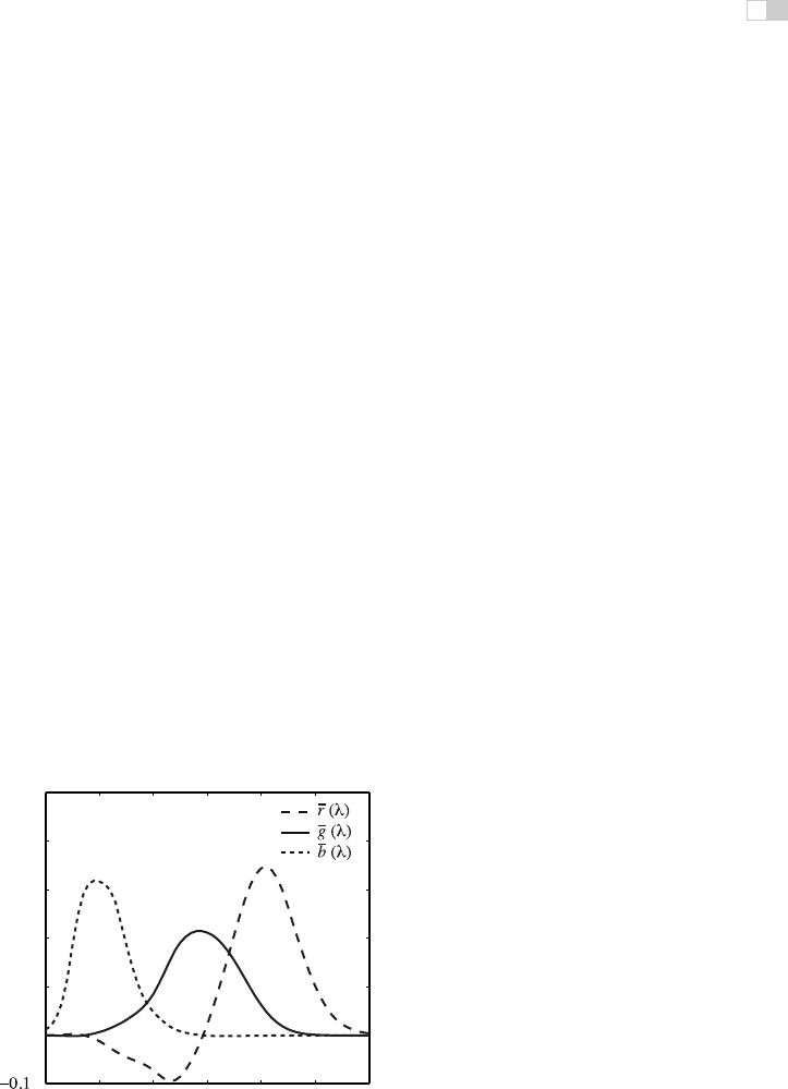
can be plotted against wavelength λ, shown in Figure 21.4.
By using a well-defined set of primary light sources, the spectral tristimulus
values lead to three color matching functions. The Commission Internationale
d’Eclairage (CIE) has defined three such primaries to be monochromatic light
sources of 435.8, 546.1, and 700 nm, respectively. With these three monochro-
matic light sources, all other visible wavelengths can be matched by adding differ-
400 450 500 550 600 650 700
0.0
0.1
0.2
0.3
0.4
0.5
wavelength (nm)
sensitivity
Figure 21.4. Spectral tristimulus values averaged over many observers. The primaries
where monochromatic light sources with wavelengths of 435.8, 546.1, and 700 nm.
i
i
i
i
i
i
i
i
538 21. Color
ent amounts of each. The amount of each required to match a given wavelength λ
is encoded in color matching functions, given by ¯r(λ), ¯g(λ),and
¯
b(λ) and plotted
in Figure 21.4. Tristimulus values associated with these color matching functions
are termed R, G,andB.
Given that we are adding light, and light cannot be negative, you may have
noticed an anomaly in Figure 21.4: to create a match for some wavelengths, it
is necessary to subtract light. Although there is no such thing as negative light,
we can use Grassmann’s laws once more, and instead of subtracting light from
the mixture of primaries, we can add the same amount of light to the color that is
being matched.
The CIE ¯r(λ), ¯g(λ),and
¯
b(λ) color matching functions allow us to determine
if a spectral distribution Φ
1
matches a second spectral distribution Φ
2
by simply
comparing the resulting tristimulus values obtained by integrating with these color
matching functions:
λ
Φ
1
(λ)¯r(λ)=
λ
Φ
2
(λ)¯r(λ),
λ
Φ
1
(λ)¯g(λ)=
λ
Φ
2
(λ)¯g(λ),
λ
Φ
1
(λ)
¯
b(λ)=
λ
Φ
2
(λ)
¯
b(λ).
Of course, a color match is only guaranteed if all three tristimulus values match.
The importance of these color matching functions lies in the fact that we are
now able to communicate and describe colors compactly by means of tristimulus
values. For a given spectral function, the CIE color matching functions provide a
precise way in which to calculate tristimulus values. As long as everybody uses
the same color matching functions, it should always be possible to generate a
match.
If the same color matching functions are not available, then it is possible to
transform one set of tristimulus values into a different set of tristimulus values
appropriate for a corresponding set of primaries. The CIE has defined one such
a transform for two specific reasons. First, in the 1930s numerical integrations
were difficult to perform, and even more so for functions that can be both posi-
tive and negative. Second, the CIE had already developed the photopic luminance
response function, CIE V (λ). It became desirable to have three integrating func-
tions, of which V (λ) is one and all three being positive over the visible range.
To create a set of positive color matching functions, it is necessary to define
imaginary primaries. In other words, to reproduce any color in the visible spec-
trum, we need light sources that cannot be physically realized. The color match-
ing functions that were settled upon by the CIE are named ¯x(λ), ¯y(λ),and¯z(λ)

i
i
i
i
i
i
i
i
21.1. Colorimetry 539
400 450 500 550 600 650 700
0.0
0.2
0.4
0.6
0.8
1.0
1.2
1.4
1.6
1.8
wavelength (nm)
sensitivity
Figure 21.5. The CIE ¯x(λ), ¯y(λ), and ¯z(λ) color matching functions.
and are shown in Figure 21.5. Note that ¯y(λ) is equal to the photopic luminance
response function V (λ) and that each of these functions is indeed positive. They
are known as the CIE 1931 standard observer.
The corresponding tristimulus values are termed X, Y ,andZ, to avoid con-
fusion with R, G,andB tristimulus values that are normally associated with real-
izable primaries. The conversion from (R, G, B) tristimulus values to (X, Y, Z)
tristimulus values is defined by a simple 3×3 transform:
⎡
⎣
X
Y
Z
⎤
⎦
=
1
0.17697
⎡
⎣
0.4900 0.3100 0.2000
0.17697 0.81240 0.01063
0.0000 0.0100 0.9900
⎤
⎦
·
⎡
⎣
R
G
B
⎤
⎦
.
To calculate tristimulus values, we typically directly integrate the standard ob-
server color matching functions with the spectrum of interest Φ(λ), rather than go
through the CIE ¯r(λ), ¯g(λ),and
¯
b(λ) color matching functions first, followed by
the above transformation. It allows us to calculate consistent color measurements
and also determine when two colors match each other.
21.1.5 Chromaticity Coordinates
Every color can be represented by a set of three tristimulus values (X, Y, Z).We
could define an orthogonal coordinate system with X, Y, and Z axes and plot each
color in the resulting 3D space. This is called a color space. The spatial extent of
the volume in which colors lie is then called the color gamut.
i
i
i
i
i
i
i
i
540 21. Color
Visualizing colors in a 3D color space is fairly difficult. Moreover, the Y -
value of any color corresponds to its luminance, by virtue of the fact that ¯y(λ)
equals V (λ). We could therefore project tristimulus values to a 2D space which
approximates chromatic information, i.e., information which is independent of
luminance. This projection is called a chromaticity diagram and is obtained by
normalization while at the same time removing luminance information:
x =
X
X + Y + Z
,
y =
Y
X + Y + Z
,
z =
Z
X + Y + Z
.
Given that x + y + z equals 1, the z-value is redundant, allowing us to plot the
x and y chromaticities against each other in a chromaticity diagram. Although x
and y by themselves are not sufficient to fully describe a color, we can use these
two chromaticity coordinates and one of the three tristimulus values, traditionally
Y , to recover the other two tristimulus values:
X =
x
y
Y,
Z =
1 − x − y
y
Y.
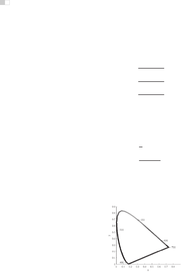
By plotting all monochromatic (spectral) colors in a chromaticity diagram,
we obtain a horseshoe-shaped curve. The points on this curve are called spectrum
loci. All other colors will generate points lying inside this curve. The spectrum
locus for the 1931 standard observer is shown in Figure 21.6. The purple line
Figure 21.6. The spectrum locus for the CIE 1931 standard observer. (See also
Plate XXVIII.)
..................Content has been hidden....................
You can't read the all page of ebook, please click here login for view all page.