
i
i
i
i
i
i
i
i
4
Ray Tracing
One of the basic tasks of computer graphics is rendering three-dimensional ob-
jects: taking a scene, or model, composed of many geometric objects arranged
in 3D space and producing a 2D image that shows the objects as viewed from
a particular viewpoint. It is the same operation that has been done for centuries
by architects and engineers creating drawings to communicate their designs to
others.
Fundamentally, rendering is a process that takesas its input a set of objects and
produces as its output an array of pixels. One way or another, rendering involves
If the output is a vector
image rather than a raster
image, rendering doesn’t
have to involve pixels, but
we’ll assume raster images
in this book.
considering how each object contributes to each pixel; it can be organized in two
general ways. In object-order rendering, each object is considered in turn, and
for each object all the pixels that it influences are found and updated. In image-
order rendering, each pixel is considered in turn, and for each pixel all the objects
that influence it are found and the pixel value is computed. You can think of
the difference in terms of the nesting of loops: in image-order rendering the “for
each pixel” loop is on the outside, whereas in object-order rendering the “for each
object” loop is on the outside.
Image-order and object-order rendering approaches can compute exactly the
same images, but they lend themselves to computing different kinds of effects
and have quite different performance characteristics. We’ll explore the compara-
In a ray tracer it is easy to
compute accurate shadows
and reflections, which are
awkward in the object-order
framework.
tive strengths of the approaches in Chapter 8 after we have discussed them both,
but, broadly speaking, image-order rendering is simpler to get working and more
flexible in the effects that can be produced, and usually (though not always) takes
much more execution time to produce a comparable image.
69
i
i
i
i
i
i
i
i
70 4. Ray Tracing
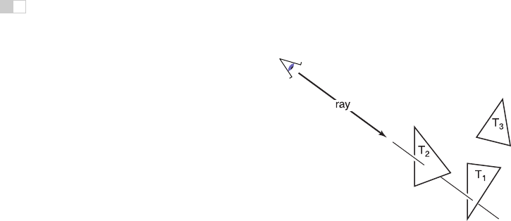
Figure 4.1. The ray is “traced” into the scene and the first object hit is the one seen through
the pixel. In this case, the triangle
T
2
is returned.
Ray tracing is an image-order algorithm for making renderings of 3D scenes,
and we’ll consider it first because it’s possible to get a ray tracer working with-
out developing any of the mathematical machinery that’s used for object-order
rendering.
4.1 The Basic Ray-Tracing Algorithm
A ray tracer works by computing one pixel at a time, and for each pixel the basic
task is to find the object that is seen at that pixel’s position in the image. Each
pixel “looks” in a different direction, and any object that is seen by a pixel must
intersect the viewing ray, a line that emanates from the viewpoint in the direction
that pixel is looking. The particular object we want is the one that intersects
the viewing ray nearest the camera, since it blocks the view of any other objects
behind it. Once that object is found, a shading computation uses the intersection
point, surface normal, and other information (depending on the desired type of
rendering) to determine the color of the pixel. This is shown in Figure 4.1, where
the ray intersects two triangles, but only the first triangle hit, T
2
, is shaded.
A basic ray tracer therefore has three parts:
1. ray generation, which computes the origin and direction of each pixel’s
viewing ray based on the camera geometry;
2. ray intersection,whichfinds the closest object intersecting the viewing ray;
3. shading, which computes the pixel color based on the results of ray inter-
section.

i
i
i
i
i
i
i
i
4.2. Perspective 71
The structure of the basic ray tracing program is:
for each pixel do
compute viewing ray
find first object hit by ray and its surface normal n
set pixel color to value computed from hit point, light, and n
This chapter covers basic methods for ray generation, ray intersection, and shad-
ing, that are sufficient for implementing a simple demonstration ray tracer. For a
really useful system, more efficient ray intersection techniques from Chapter 12
need to be added, and the real potential of a ray tracer will be seen with the more
advanced shading methods from Chapter 10 and the additional rendering tech-
niques from Chapter 13.
4.2 Perspective
The problem of representing a 3D object or scene with a 2D drawing or paint-
ing was studied by artists hundreds of years before computers. Photographs also
represent 3D scenes with 2D images. While there are many unconventional ways
to make images, from cubist painting to fish-eye lenses (Figure 4.2) to peripheral
cameras, the standard approach for both art and photography, as well as computer
graphics, is linear perspective, in which 3D objects are projected onto an image
plane in such a way that straight lines in the scene become straight lines in the
image.
Figure 4.2. An image
takenwithafisheyelensis
not a linear perspective im-
age.
Photo courtesy Philip
Greenspan.
The simplest type of projection is parallel projection, in which 3D points are
mapped to 2D by moving them along a projection direction until they hit the
image plane (Figures 4.3–4.4). The view that is produced is determined by the
choice of projection direction and image plane. If the image plane is perpendicular
axis-aligned
orthographic
orthographic
Figure 4.3. When projection lines are parallel and perpendicular to the image plane, the
resulting views are called orthographic.

i
i
i
i
i
i
i
i
72 4. Ray Tracing
perspective
oblique
Figure 4.4. A parallel projection that has the image plane at an angle to the projection di-
rection is called oblique (right). In perspective projection, the projection lines all pass through
the viewpoint, rather than being parallel (left). The illustrated perspective view is non-oblique
because a projection line drawn through the center of the image would be perpendicular to
the image plane.
to the view direction, the projection is called orthographic; otherwise it is called
oblique.
Some books reserve “or-
thographic” for projection
directions that are parallel
to the coordinate axes.
Parallel projections are often used for mechanical and architectural drawings
because they keep parallel lines parallel and they preserve the size and shape of
planar objects that are parallel to the image plane.
The advantages of parallel projection are also its limitations. In our everyday
experience (and even more so in photographs) objects look smaller as they get
farther away, and as a result parallel lines receding into the distance do not ap-
pear parallel. This is because eyes and cameras don’t collect light from a single
viewing direction; they collect light that passes through a particular viewpoint.
As has been recognized by artists since the Renaissance, we can produce natural-
Figure 4.5. In three-point perspective, an artist picks “vanishing points” where parallel
lines meet. Parallel horizontal lines will meet at a point on the horizon. Every set of parallel
lines has its own vanishing points. These rules are followed automatically if we implement
perspective based on the correct geometric principles.

i
i
i
i
i
i
i
i
4.3. Computing Viewing Rays 73
looking views using perspective projection: we simply project along lines that
pass through a single point, the viewpoint, rather than along parallel lines (Fig-
ure 4.4). In this way objects farther from the viewpoint naturally become smaller
when they are projected. A perspective view is determined by the choice of view-
point (rather than projection direction) and image plane. As with parallel views
there are oblique and non-obliqueperspective views; the distinction is made based
on the projection direction at the center of the image.
You may have learned about the artistic conventions of three-point perspec-
tive, a system for manually constructing perspective views (Figure 4.5). A sur-
prising fact about perspective is that all the rules of perspective drawing will be
followed automatically if we follow the simple mathematical rule underlying per-
spective: objects are projected directly toward the eye, and they are drawn where
they meet a view plane in front of the eye.
4.3 Computing Viewing Rays
From the previous section, the basic tools of ray generation are the viewpoint (or
view direction, for parallel views) and the image plane. There are many ways to
work out the details of camera geometry; in this section we explain one based
on orthonormal bases that supports normal and oblique parallel and orthographic
views.
In order to generate rays, we first need a mathematical representation for a ray.
A ray is really just an origin point and a propagation direction; a 3D parametric
line is ideal for this. As discussed in Section 2.5.7, the 3D parametric line from
the eye e to a point s on the image plane (Figure 4.6) is given by
Figure 4.6. The ray from
the eye to a point on the im-
age plane.
p(t)=e + t(s − e).
This should be interpreted as, “we advance from e along the vector (s − e) a
fractional distance t to find the point p.” So given t, we can determine a point p.
The point e is the ray’s origin,ands − e is the ray’s direction.
Caution: we are overload-
ing the variable
t
,whichis
the ray parameter and also
the
v
-coordinate of the top
edge of the image.
Note that p(0) = e,andp(1) = s, and more generally, if 0 <t
1
<t
2
,then
p(t
1
) is closer to the eye than p(t
2
). Also, if t<0,thenp(t) is “behind” the eye.
These facts will be useful when we search for the closest object hit by the ray that
is not behind the eye.
To compute a viewing ray, we need to know e (which is given) and s. Finding
s may seem difficult, but it is actually straightforward if we look at the problem
in the right coordinate system.
..................Content has been hidden....................
You can't read the all page of ebook, please click here login for view all page.