
i
i
i
i
i
i
i
i
7.3. Perspective Projection 151
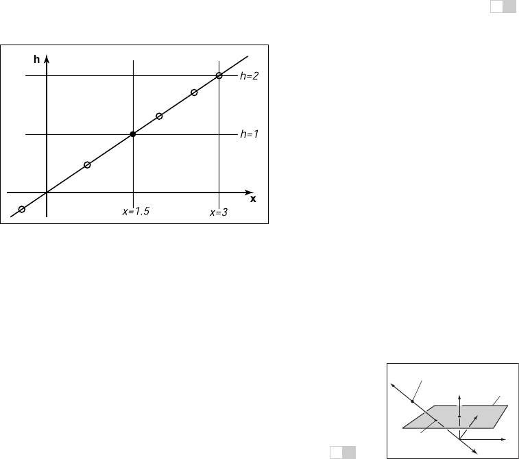
Figure 7.10. The point
x
= 1.5 is represented by any point on the line
x
=1.5
h
,such
as points at the hollow circles. However, before we interpret
x
as a conventional Cartesian
coordinate, we first divide by
h
to get (
x,h
) = (1.5,1) as shown by the black point.
Example. In 1D homogeneous coordinates, in which we use 2-vectors to repre-
sent points on the real line, we could represent the point (1.5) using the homoge-
neous vector [1.51]
T
, or any other point on the line x =1.5h in homogeneous
space. (See Figure 7.10.)
In 2D homogeneouscoordinates, in which we use 3-vectorsto represent points
in the plane, we could represent the point (−1, −0.5) using the homogeneous
vector [−2; −1; 2]
T
, or any other point on the line x = α[−1 − 0.51]
T
.Any
homogeneous vector on the line can be mapped to the line’s intersection with the
plane w =1to obtain its Cartesian coordinates. (See Figure 7.11.)
x
y
w
(–1, –.5, 1)
(–2, –1, 2)
αv
v
w = 1
Figure 7.11. A point in
homogeneous coordinates
is equivalent to any other
point on the line through
it and the origin, and nor-
malizing the point amounts
to intersecting this line with
the plane
w
=1.
It’s fine to transform homogeneous vectors as many times as needed, with-
out worrying about the value of the w-coordinate—in fact, it is fine if the w-
coordinate is zero at some intermediate phase. It is only when we want the ordi-
nary Cartesian coordinates of a point that we need to normalize to an equivalent
point that has w =1, which amounts to dividing all the coordinates by w.Once
we’ve done this we are allowed to read off the (x, y, z)-coordinates from the first
three components of the homogeneous vector.
7.3 Perspective Projection
The mechanism of projective transformations makes it simple to implement the
division by z required to implement perspective. In the 2D example shown in Fig-
ure 7.8, we can implement the perspective projectionwith a matrix transformation

i
i
i
i
i
i
i
i
152 7. Viewing
as follows:
y
s
1
∼
d 00
010
⎡
⎣
y
z
1
⎤
⎦
.
This transforms the 2D homogeneous vector [y; z;1]
T
to the 1D homogeneous
vector [dy z]
T
, which represents the 1D point (dy/z) (because it is equivalent to
the 1D homogeneous vector [dy/z 1]
T
. This matches Equation (7.5).
For the “official” perspective projection matrix in 3D, we’ll adopt our usual
convention of a camera at the origin facing in the −z direction, so the distance
of the point (x, y, z) is −z. As with orthographic projection, we also adopt the
notion of near and far planes that limit the range of distances to be seen. In this
context, we will use the near plane as the projection plane, so the image plane
distance is −n.
Remember,
n
< 0.
The desired mapping is then y
s
=(n/z)y, and similarly for x. This transfor-
mation can be implemented by the perspective matrix:
P =
⎡
⎢
⎢
⎣
n 00 0
0 n 00
00n + f − fn
00 1 0
⎤
⎥
⎥
⎦
.
The first, second, and fourth rows simply implement the perspective equation.
The third row, as in the orthographic and viewport matrices, is designed to bring
the z-coordinate “along for the ride” so that we can use it later for hidden surface
removal. In the perspective projection, though, the addition of a non-constant
denominator prevents us from actually preserving the value of z—it’s actually
impossible to keep z from changing while getting x and y to do what we need
them to do. Instead we’ve opted to keep z unchanged for points on the near or far
More on this later.
planes.
There are many matrices that could function as perspective matrices, and all
of them non-linearly distort the z-coordinate. This specific matrix has the nice
properties shown in Figures 7.12 and 7.13; it leaves points on the (z = n)-
plane entirely alone, and it leaves points on the (z = f)-plane while “squishing”
them in x and y by the appropriate amount. The effect of the matrix on a point
(x, y, z) is
P
⎡
⎢
⎢
⎢
⎢
⎣
x
y
z
1
⎤
⎥
⎥
⎥
⎥
⎦
=
⎡
⎢
⎢
⎢
⎢
⎣
x
y
z
n+f
n
− f
z
n
⎤
⎥
⎥
⎥
⎥
⎦
∼
⎡
⎢
⎢
⎢
⎢
⎣
nx
z
ny
z
n + f −
fn
z
1
⎤
⎥
⎥
⎥
⎥
⎦
.
i
i
i
i
i
i
i
i
7.3. Perspective Projection 153
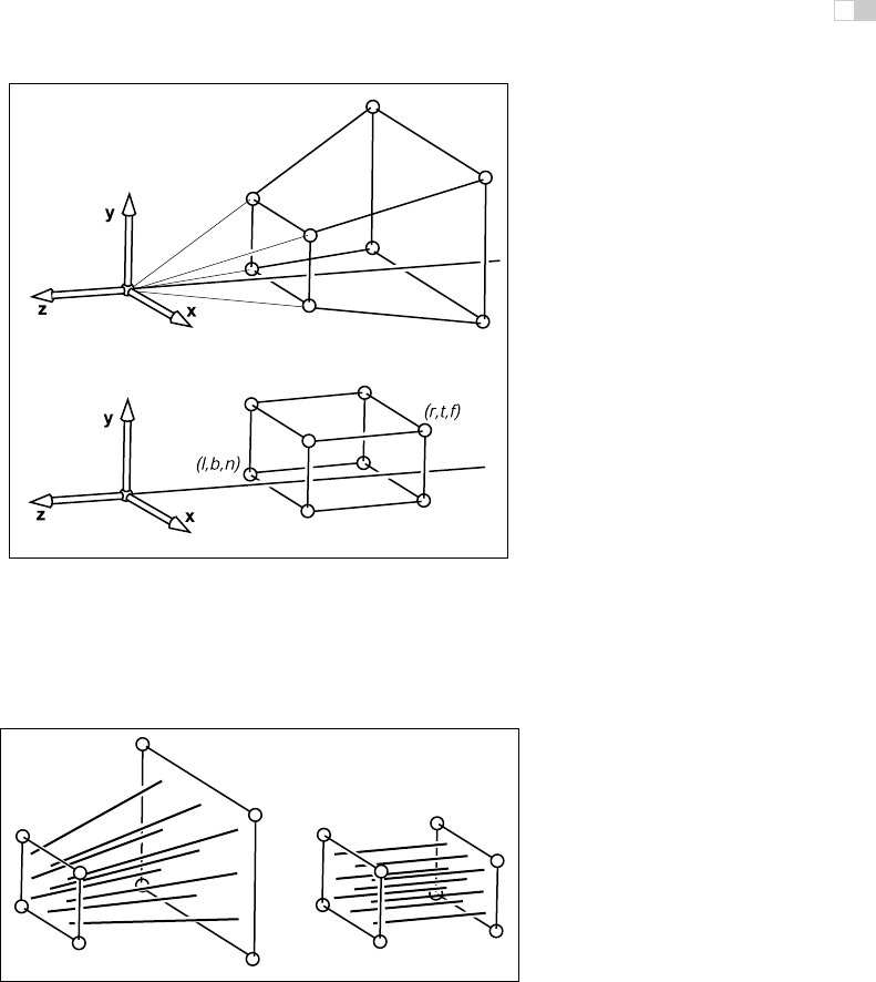
Figure 7.12. The perspective projection leaves points on the
z=n
plane unchanged and
maps the large
z=f
rectangle at the back of the perspective volume to the small
z=f
rectangle at the back of the orthographic volume.
Figure 7.13. The perspective projection maps any line through the origin/eye to a line
parallel to the
z
-axis and without moving the point on the line at
z=n
.

i
i
i
i
i
i
i
i
154 7. Viewing
As you can see, x and y are scaled and, more importantly, divided by z. Because
both n and z (inside the view volume) are negative, there are no “flips” in x
and y. Although it is not obvious (see the exercise at the end of the chapter),
the transform also preserves the relative order of z values between z = n and
z = f, allowing us to do depth ordering after this matrix is applied. This will be
important later when we do hidden surface elimination.
Sometimes we will want to take the inverse of P, for example to bring a screen
coordinate plus z back to the original space, as we might want to do for picking.
The inverse is
P
−1
=
⎡
⎢
⎢
⎣
1
n
00 0
0
1
n
00
00 0 1
00−
1
fn
n+f
fn
⎤
⎥
⎥
⎦
.
Since multiplying a homogeneous vector by a scalar does not change its meaning,
the same is true of matrices that operate on homogeneous vectors. So we can
write the inverse matrix in a prettier form by multiplying through by nf:
P
−1
=
⎡
⎢
⎢
⎣
f 00 0
0 f 00
00 0 fn
00−1 n + f
⎤
⎥
⎥
⎦
.
This matrix is not literally
the inverse of the matrix
P, but the transformation
it describes
is
the inverse
of the transformation de-
scribed by P.
Taken in the context of the orthographic projection matrix M
orth
in Equa-
tion (7.3), the perspectivematrix simply maps the perspective view volume (which
is shaped like a slice, or frustum, of a pyramid) to the orthographic view volume
(which is an axis-aligned box). The beauty of the perspective matrix is, that once
we apply it, we can use an orthographic transform to get to the canonical view
volume. Thus, all of the orthographic machinery applies, and all that we have
added is one matrix and the division by w. It is also heartening that we are not
“wasting” the bottom row of our four by four matrices!
Concatenating P with M
orth
results in the perspective projection matrix,
M
per
= M
orth
P.
One issue, however, is: How are l,r,b,t determined for perspective? They
identify the “window” through which we look. Since the perspective matrix does
not change the values of x and y on the (z = n)-plane, we can specify (l, r,b, t)
on that plane.
To integrate the perspective matrix into our orthographic infrastructure, we
simply replace M
orth
with M
per
, which inserts the perspective matrix P after the
camera matrix M
cam
has been applied but before the orthographic projection. So

i
i
i
i
i
i
i
i
7.3. Perspective Projection 155
the full set of matrices for perspective viewing is
M = M
vp
M
orth
PM
cam
.
The resulting algorithm is:
compute M
vp
compute M
per
compute M
cam
M = M
vp
M
per
M
cam
for each line segment (a
i
, b
i
) do
p = Ma
i
q = Mb
i
drawline(x
p
/w
p
,y
p
/w
p
,x
q
/w
q
,y
q
/w
q
)
Note that the only change other than the additional matrix is the divide by the
homogeneous coordinate w.
Multiplied out, the matrix M
per
looks like this:
M
per
=
⎡
⎢
⎢
⎢
⎢
⎢
⎢
⎢
⎢
⎣
2n
r−l
0
l+r
l−r
0
0
2n
t−b
b+t
b−t
0
00
f+n
n−f
2fn
f−n
00 1 0
⎤
⎥
⎥
⎥
⎥
⎥
⎥
⎥
⎥
⎦
.
This or similar matrices often appear in documentation, and they are less mysteri-
ous when one realizes that they are usually the product of a few simple matrices.
Example. Many APIs such as OpenGL (Shreineret al., 2004) use the same canon-
ical view volume as presented here. They also usually have the user specify the
absolute values of n and f. The projection matrix for OpenGL is
M
OpenGL
=
⎡
⎢
⎢
⎢
⎢
⎢
⎢
⎢
⎢
⎢
⎣
2|n|
r−l
0
r+l
r−l
0
0
2|n|
t−b
t+b
t−b
0
00
|n|+|f|
|n|−|f|
2|f||n|
|n|−|f|
00 −10
⎤
⎥
⎥
⎥
⎥
⎥
⎥
⎥
⎥
⎥
⎦
.
Other APIs set n and f to 0 and 1, respectively. Blinn (J. Blinn, 1996) recom-
mends making the canonical view volume [0, 1]
3
for efficiency. All such decisions
will change the the projection matrix slightly.
..................Content has been hidden....................
You can't read the all page of ebook, please click here login for view all page.