

i
i
i
i
i
i
i
i
11.3. Texture Mapping for Rasterized Triangles 253
texture coordinates in screen space results in incorrect images, as shown for the
grid texture shown in Figure 11.11. Because things in perspective get smaller as
the distance to the viewer increases, the lines that are evenly spaced in 3D should
compress in 2D image space. More careful interpolation of texture coordinates is
needed to accomplish this.
Figure 11.11. Left: correct
perspective. Right: interpo-
lation in screen space.
11.3.1 Perspective Correct Textures
We can implement texture mapping on triangles by interpolating the (u, v) coor-
dinates, modifying the rasterization method of Section 8.1.2, but this results in the
problem shown at the right of Figure 11.11. A similar problem occurs for triangles
if screen space barycentric coordinates are used as in the following rasterization
code:
for all x do
for all y do
compute (α, β, γ) for (x, y)
if α ∈ (0, 1) and β ∈ (0, 1) and γ ∈ (0, 1) then
t = αt
0
+ βt
1
+ γt
2
drawpixel (x, y) with color texture(t) for a solid texture
or with texture(β,γ) for a 2D texture.
This code will generate images, but there is a problem. To unravel the basic prob-
lem, let’s consider the progression from world space q to homogeneouspoint r to
homogenized point s:
⎡
⎢
⎢
⎣
x
q
y
q
z
q
1
⎤
⎥
⎥
⎦
transform
−−−−−→
⎡
⎢
⎢
⎣
x
r
y
r
z
r
h
r
⎤
⎥
⎥
⎦
homogenize
−−−−−−− →
⎡
⎢
⎢
⎣
x
r
/h
r
y
r
/h
r
z
r
/h
r
1
⎤
⎥
⎥
⎦
≡
⎡
⎢
⎢
⎣
x
s
y
s
z
s
1
⎤
⎥
⎥
⎦
.
If we use screen space, we are interpolating in s.However,wewouldliketobe
interpolating in space q or r, where the homogeneous division has not yet non-
linearly distorted the barycentric coordinates of the triangle.
The key observation is that 1/h
r
is interpolated with no distortion. Likewise,
so is u/h
r
and v/h
r
. In fact, so is k/h
r
,wherek is any quantity that varies
linearly across the triangle. Recall from Section 7.4 that if we transform all points
along the line segment between points q and Q and homogenize, we have
s +
h
R
t
h
r
+ t(h
R
− h
r
)
(S − s),

i
i
i
i
i
i
i
i
254 11. Texture Mapping
but if we linearly interpolate in the homogenized space we have
s + a(S − s).
Although those lines sweep out the same points, typically a = t for the same
points on the line segment. However, if we interpolate 1/h,wedo get the same
answer regardless of which space we interpolate in. To see this is true, confirm
(Exercise 2):
1
h
r
+
h
R
t
h
r
+ t(h
R
− h
r
)
1
h
R
−
1
h
r
=
1
h
r
+ t
1
h
R
−
1
h
r
(11.4)
This ability to interpolate 1/h linearly with no error in the transformed space
allows us to correctly texture triangles. Perhaps the least confusing way to deal
with this distortion is to compute the world space barycentric coordinates of the
triangle (β
w
,γ
w
) in terms of screen space coordinates (β,γ). We note that β
s
/h
and γ
s
/h can be interpolated linearly in screen space. For example, at the screen
space position associated with screen space barycentric coordinates (β, γ),we
can interpolate β
w
/h without distortion. Because β
w
=0at vertex 0 and vertex
2, and β
w
=1at vertex 1, we have
β
s
h
=
0
h
0
+ β
1
h
1
−
0
h
0
+ γ
0
h
2
−
0
h
0
. (11.5)
Because of all the zero terms, Equation (11.5) is fairly simple. However, to get
β
w
from it, we must know h. Because we know 1/h is linear in screen space, we
have
1
h
=
1
h
0
+ β
1
h
1
−
1
h
0
+ γ
1
h
2
−
1
h
0
. (11.6)
Dividing Equation (11.5) by Equation (11.6) gives
β
w
=
β
h
1
1
h
0
+ β
1
h
1
−
1
h
0
+ γ
1
h
2
−
1
h
0
.
Multiplying numerator and denominator by h
0
h
1
h
2
and doing a similar set of
manipulations for the analogous equations in γ
w
gives
β
w
=
h
0
h
2
β
h
1
h
2
+ h
2
β(h
0
− h
1
)+h
1
γ(h
0
− h
2
)
,
γ
w
=
h
0
h
1
γ
h
1
h
2
+ h
2
β(h
0
− h
1
)+h
1
γ(h
0
− h
2
)
.
(11.7)
Note that the two denominators are the same.
i
i
i
i
i
i
i
i
11.4. Bump Textures 255
For triangles that use the perspective matrix from Chapter 7, recall that w =
z/n where z is the distance from the viewer perpendicular to the screen. Thus,
for that matrix 1/z also varies linearly. We can use this fact to modify our
scan-conversion code for three points t
i
=(x
i
,y
i
,z
i
,h
i
) that have been passed
through the viewing matrices, but have not been homogenized:
Compute bounds for x = x
i
/h
i
and y = y
i
/h
i
for all x do
for all y do
compute (α, β, γ) for (x, y)
if (α ∈ [0, 1] and β ∈ [0, 1] and γ ∈ [0, 1]) then
d = h
1
h
2
+ h
2
β(h
0
− h
1
)+h
1
γ(h
0
− h
2
)
β
w
= h
0
h
2
β/d
γ
w
= h
0
h
1
γ/d
α
w
=1− β
w
− γ
w
u = α
w
u
0
+ β
w
u
1
+ γ
w
u
2
v = α
w
v
0
+ β
w
v
1
+ γ
w
v
2
drawpixel (x, y) with color texture(u, v)
For solid textures, just recall that by the definition of barycentric coordinates
p =(1−β
w
− γ
w
)p
0
+ β
w
p
1
+ γ
w
p
2
,
where p
i
are the world space vertices. Then, just call a solid texture routine for
point p.
11.4 Bump Textures
Although we have only discussed changing reflectance using texture, you can also
change the surface normal to give an illusion of fine-scale geometry on the sur-
face. We can apply a bump map that perturbs the surface normal
(J. F. Blinn, 1978).
One way to do this is:
vector3 n = surfaceNormal(x)
n += k
1
∗ vectorTurbulence(k
2
∗ x)
return t ∗ s0+(1− t) ∗ s1
This is shown in Figure 11.12.
To implement vectorTurbulence,wefirst need vectorNoise which produces a
simple spatially-varying 3D vector:
n
v
(x, y, z)=
x+1
i=x
y+1
j=y
z+1
k=z
Γ
ijk
ω(x)ω(y)ω(z).
i
i
i
i
i
i
i
i
256 11. Texture Mapping
Then, vectorTurbulence is a direct analog of turbulence: sum a series of scaled
versions of vectorNoise.
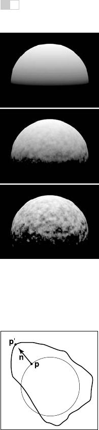
Figure 11.12. Vector tur-
bulence on a sphere of ra-
dius 1.6. Lighting directly
from above. Top: k
1
=0.
Middle: k
1
= 0.08, k
2
=8.
Bottom: k
1
= 0.24, k
2
=8.
11.5 Displacement Mapping
One problem with Figure 11.12 is that the bumps neither cast shadows nor affect
the silhouette of the object. These limitations occur because we are not really
changing any geometry. If we want more realism, we can apply a displacement
map (Cook et al., 1987). A displacement map actually changes the geometry
using a texture. A common simplification is that the displacement will be in the
direction of the surface normal.
Figure 11.13. The points
p on the circle are each dis-
placed in the direction of n
by the function
f
(p).If
f
is
continuous, then the result-
ing points p
form a contin-
uous surface.
If we take all points p on a surface, with associated surface normal vectors n,
then we can make a new surface using a 3D texture d(p):
p
= p + f(p)n.
This concept is shown in Figure 11.13.
Displacement mapping is straightforward to implement in a z-buffer code by
storing the surface to be displaced as a fine mesh of many triangles. Each vertex
in the mesh can then be displaced along the normal vector direction. This results
in large models, but it is quite robust.
11.6 Environment Maps
Often we would like to have a texture-mapped background and for objects to
have specular reflections of that background. This can be accomplished using
environment maps (J. F. Blinn, 1976). An environment map can be implemented
as a background function that takes in a viewing direction b and returns a RGB
color from a texture map. There are many ways to store environment maps. For
example, we can use a spherical table indexed by spherical coordinates. In this
section, we will instead describe a cube-based table with six square texture maps,
often called a cube map.
The basic idea of a cube map is that we have an infinitely large cube with
a texture on each face. Because the cube is large, the origin of a ray does not
change what the ray “sees.” This is equivalent to an arbitrarily-sized cube that is
queried by a ray whose origin is at the Cartesian origin. As an example of how
a given direction b is converted to (u, v) coordinates, consider the right face of

i
i
i
i
i
i
i
i
11.6. Environment Maps 257
Figure 11.14. The cube map has six axis-aligned textures that store the background. The
right face contains a single texture.
Figure 11.14. Here we have x
b
as the maximum magnitude component. In that
case, we can compute (u, v) for that texture to be
u =
y + x
2x
,
v =
z + x
2x
.
There are analogous formulas for the other five faces.
So for any reflection ray a + tb we return cubemap(b) for the background
color. In a z-buffer implementation, we need to perform this calculation on a
pixel-by-pixel basis. If at a given pixel we know the viewing direction c and the
surface normal vector n, we can compute the reflected direction b (Figure 11.15).
We can do this by modifying Equation (10.6) to get
b = −c +
2(c ·n)n
c
2
. (11.8)
Here the denominator of the fraction accounts for the fact that c may not be a unit
Figure 11.15. The vector
b is the reflection of vector
c with respect to the surface
normal n.
vector. Because we need to know b at each pixel, we can either compute b at
each triangle vertex and interpolate b in a perspective correct manner, or we can
interpolate n and compute b for each pixel. This will allow us to call cubemap(b)
at each pixel.
..................Content has been hidden....................
You can't read the all page of ebook, please click here login for view all page.