
i
i
i
i
i
i
i
i
628 24. Global Illumination
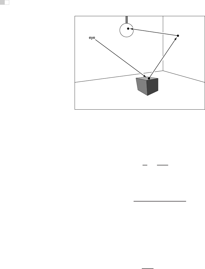
Figure 24.4. In path tracing, a ray is followed through a pixel from the eye and scattered
through the scene until it hits a luminaire.
We use Monte Carlo integration to approximate the solution to this equation for
each viewing ray. Recall from Section 14.3, that we can use random samples to
approximate an integral:
x∈S
g(x)dμ ≈
1
N
N
i=1
g(x
i
)
p(x
i
)
,
where the x
i
are random points with probability density function p. If we apply
this directly to the transport equation with N =1we get
L
s
(k
o
) ≈ L
e
(k
o
)+
ρ(k
i
, k
o
)L
f
(k
i
)cosθ
i
dσ
i
p(k
i
)
.
So if we have a way to select random directions k
i
with a known density p,we
can get an estimate. The catch is that L
f
(k
i
) is itself an unknown. Fortunately
we can apply recursion and use a statistical estimate for L
f
(k
i
) by sending a ray
in that direction to find the surface seen in that direction. We end when we hit
a luminaire and L
e
is non-zero (Figure 24.4). This method assumes lights have
zero reflectance, or we would continue to recurse.
In the case of a Lambertian BRDF (ρ = R/π), we can use a cosine density
function:
p(k
i
)=
cos θ
i
π
.
i
i
i
i
i
i
i
i
24.3. Accurate Direct Lighting 629
A direction with this density can be chosen according to Equation (24.3). This
allows some cancellation of cosine terms in our estimate:
L
s
(k
o
) ≈ L
e
(k
o
)+RL
f
(k
i
).
In pseudocode such a path tracer for Lambertian surfaces would operate just
like the ray tracers described in Chapter 4, but the raycolor function would be
modified:
RGB raycolor(ray a + tb, int depth)
if (ray hits at some point c ) then
RGB c = L
e
(−b)
if (depth < maxdepth) then
compute random direction d
return c + R raycolor(c + sd,depth+1)
else
return background color
This will result in a very noisy image unless either large luminaires or very large
numbers of samples are used. Note the color of the luminaires must be well above
one (sometimes thousands or tens of thousands) to make the surfaces have final
colors near one, because only those rays that hit a luminaire by chance will make
a contribution, and most rays will contribute only a color near zero. To generate
the random direction d, we use the same technique as we do in particle tracing
(see Equation (24.2)).
In the general case we might want to use spectral colors or use a more general
BRDF. In practice, we should have the material class contain member functions
to compute a random direction as well as compute the p associated with that
direction. This way materials can be added transparently to an implementation.
24.3 Accurate Direct Lighting
This section presents a more physically-based method of direct lighting than
Chapter 10. These methods will be useful in making global illumination algo-
rithms more efficient. The key idea is to send shadow rays to the luminaires as
described in Chapter 4, but to do so with careful bookkeeping based on the trans-
port equation from the previous chapter. The global illumination algorithms can
be adjusted to make sure they compute the direct component exactly once. For
example, in particle tracing, particles coming directly from the luminaire would
not be logged, so the particles would only encode indirect lighting. This makes

i
i
i
i
i
i
i
i
630 24. Global Illumination
nice looking shadows much more efficiently than computing direct lighting in the
context of global illumination.
24.3.1 Mathematical Framework
To calculate the direct light from one luminaire (light emitting object) onto a non-
emitting surface, we solve a form of the transport equation from Section 20.2:
L
s
(x, k
o
)=
all x
ρ(k
i
, k
o
)L
e
(x
, −k
i
)v(x, x
)cosθ
i
cos θ
x − x
2
dA
. (24.4)
Recall that L
e
is the emitted radiance of the source, v is a visibility function that
is equal to 1 if x “sees” x
and zero otherwise, and the other variables are as
illustrated in Figure 24.5.
If we are to sample Equation (24.4) using Monte Carlo integration, we need
Figure 24.5. The direct
lighting terms for Equa-
tion (24.4).
to pick a random point x
on the surface of the luminaire with density function p
(so x
∼ p). Just plugging into Equation (14.5) with one sample yields
L
s
(x, k
o
) ≈
ρ(k
i
, k
o
)L
e
(x
, −k
i
)v(x, x
)cosθ
i
cos θ
p(x
)x − x
2
. (24.5)
If we pick a uniform random point on the luminaire, then p =1/A,whereA is
the area of the luminaire. This gives
L
s
(x, k
o
) ≈
ρ(k
i
, k
o
)L
e
(x
, −k
i
)v(x, x
)A cos θ
i
cos θ
x − x
2
. (24.6)
We can use Equation (24.6) to sample planar (e.g., rectangular) luminaires in a
straightforward fashion. We simply pick a random point on each luminaire.
The code for one luminaire is:
color directLight( x, k
o
, n)
pick random point x
with normal vector n
on light
d = x
− x
k
i
= d/d
if (ray x + td has no hits for t<1 − ) then
return ρ(k
i
, k
o
)L
e
(x
, −k
i
)(n · d)(−n
·d)/d
4
else
return 0
The above code needs some extra tests such as clamping the cosines to zero if
they are negative. Note that the term d
4
comes from the distance squared term
i
i
i
i
i
i
i
i
24.3. Accurate Direct Lighting 631
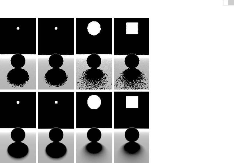
Figure 24.6. Various soft shadows on a backlit sphere with a square and an area light
source. Top: 1 sample. Bottom: 100 samples. Note that the shape of the light source is less
important than its size in determining shadow appearance.
and the two cosines, e.g., n · d = dcos θ because d is not necessarily a unit
vector.
Several examples of soft shadows are shown in Figure 24.6.
24.3.2 Sampling a Spherical Luminaire
Though a sphere with center c and radius R can be sampled using Equation (24.6),
this sampling will yield a very noisy image because many samples will be on the
back of the sphere, and the cos θ
term varies so much. Instead, we can use a more
complex p(x
) to reduce noise.
The first non-uniform density we might try is p(x
) ∝ cos θ
. This turns out to
be just as complicated as sampling with p(x
) ∝ cos θ
/x
−x
2
, so we instead
discuss that here. We observe that sampling on the luminaire this way is the
same as using a constant density function q(k
i
)=const defined in the space of
directions subtended by the luminaire as seen from x. We now use a coordinate

i
i
i
i
i
i
i
i
632 24. Global Illumination
Figure 24.7. Geometry for direct lighting at point x from a spherical luminaire.
system defined with x at the origin, and a right-handed orthonormal basis with
w =(c − x)/c − x,andv =(w × n)/(w × n) (see Figure 24.7). We
also define (α, φ) to be the azimuthal and polar angles with respect to the uvw
coordinate system.
The maximum α that includes the spherical luminaire is given by
α
max
=arcsin
R
x − c
= arccos
"
1 −
R
x − c
2
.
Thus, a uniform density (with respect to solid angle) within the cone of directions
subtended by the sphere is just the reciprocal of the solid angle 2π(1 −cos α
max
)
subtended by the sphere:
q(k
i
)=
1
2π
&
1 −
1 −
R
x−c
2
'
.
And we get
cos α
φ
=
⎡
⎣
1 − ξ
1
+ ξ
1
1 −
R
x−c
2
2πξ
2
⎤
⎦
.
This gives us the direction k
i
.Tofind the actual point, we need to find the first
point on the sphere in that direction. The ray in that direction is just (x + tk
i
),
..................Content has been hidden....................
You can't read the all page of ebook, please click here login for view all page.