

i
i
i
i
i
i
i
i
308 13. More Ray Tracing
Figure 13.5. The ray intersection problem in the two spaces are just simple transforms of
each other. The object is specified as a sphere plus matrix M. The ray is specified in the
transformed (world) space by location a and direction b.
2. many transformed objects can share the same untransformed object thus
reducing storage, e.g., a traffic jam of cars, where individual cars are just
transforms of a few base (untransformed) models.
As discussed in Section 6.2.2, surface normal vectors transform differently.
With this in mind and using the concepts illustrated in Figure 13.5, we can
determine the intersection of a ray and an object transformed by matrix M.Ifwe
create an instance class of type surface, we need to create a hit
function:
instance::hit(ray a + tb, real t
0
, real t
1
, hit-record rec)
ray r
= M
−1
a + tM
−1
b
if (base-object→hit(r
, t
0
, t
1
,rec)) then
rec.n =(M
−1
)
T
rec.n
return true
else
return false
An elegant thing about this function is that the parameter rec.t does not need to
be changed, because it is the same in either space. Also note that we need not
compute or store the matrix M.

i
i
i
i
i
i
i
i
13.3. Constructive Solid Geometry 309
This brings up a very important point: the ray direction b must not be re-
stricted to a unit-length vector, or none of the infrastructure above works. For this
reason, it is useful not to restrict ray directions to unit vectors.
13.3 Constructive Solid Geometry
One nice thing about ray tracing is that any geometric primitive whose intersection
with a 3D line can be computed can be seamlessly added to a ray tracer. It turns
out to also be straightforward to add constructive solid geometry (CSG) to a ray
tracer (Roth, 1982). The basic idea of CSG is to use set operations to combine
solid shapes. These basic operations are shown in Figure 13.6. The operations
can be viewed as set operations. For example, we can consider C the set of all
points in the circle and S the set of all points in the square. The intersection
Figure 13.6. The ba-
sic CSG operations on a 2D
circle and square.
operation C ∩ S is the set of all points that are both members of C and S.The
other operations are analogous.
Although one can do CSG directly on the model, if all that is desired is an
image, we do not need to explicitly change the model. Instead, we perform the set
operations directly on the rays as they interact with a model. To make this natural,
we find all the intersections of a ray with a model rather than just the closest. For
example, a ray a + tb might hit a sphere at t =1and t =2. In the context
of CSG, we think of this as the ray being inside the sphere for t ∈ [1, 2].We
can compute these “inside intervals” for all of the surfaces and do set operations
on those intervals (recall Section 2.1.2). This is illustrated in Figure 13.7, where
the hit intervals are processed to indicate that there are two intervals inside the
difference object. The first hit for t>0 is what the ray actually intersects.
In practice, the CSG intersection routine must maintain a list of intervals.
When the first hitpoint is determined, the material property and surface normal is
that associated with the hitpoint. In addition, you must pay attention to precision
issues because there is nothing to prevent the user from taking two objects that
abut and taking an intersection. This can be made robust by eliminating any
interval whose thickness is below a certain tolerance.
Figure 13.7. Intervals are
processed to indicate how
the ray hits the composite
object.
13.4 Distribution Ray Tracing
For some applications, ray-traced images are just too “clean.” This effect can be
mitigated using distribution ray tracing (Cook et al., 1984) . The conventionally
ray-traced images look clean, because everything is crisp; the shadows are per-

i
i
i
i
i
i
i
i
310 13. More Ray Tracing
fectly sharp, the reflections have no fuzziness, and everything is in perfect focus.
Figure 13.8. Sixteen reg-
ular samples for a single
pixel.
Sometimes we would like to have the shadows be soft (as they are in real life), the
reflections be fuzzy as with brushed metal, and the image have variable degrees of
focus as in a photograph with a large aperture. While accomplishing these things
from first principles is somewhat involved (as is developed in Chapter 24), we
can get most of the visual impact with some fairly simple changes to the basic ray
tracing algorithm. In addition, the framework gives us a relatively simple way to
antialias (recall Section 8.3) the image.
13.4.1 Antialiasing
Figure 13.9. Asimple
scene rendered with one
sample per pixel (lower left
half) and nine samples per
pixel (upper right half).
Recall that a simple way to antialias an image is to compute the average color
for the area of the pixel rather than the color at the center point. In ray tracing,
our computational primitive is to compute the color at a point on the screen. If
we average many of these points across the pixel, we are approximating the true
average. If the screen coordinates bounding the pixel are [i, i +1]× [j, j +1],
then we can replace the loop:
for each pixel (i, j) do
c
ij
= ray-color(i +0.5,j+0.5)
with code that samples on a regular n × n grid of samples within each pixel:
for each pixel (i, j) do
c =0
for p =0to n − 1 do
for q =0to n − 1 do
c = c + ray-color(i +(p +0.5)/n, j +(q +0.5)/n)
c
ij
= c/n
2
This is usually called regular sampling. The 16 sample locations in a pixel for
n =4are shown in Figure 13.8. Note that this produces the same answer as
rendering a traditional ray-traced image with one sample per pixel at n
x
n by n
y
n
resolution and then averaging blocks of n by n pixels to get a n
x
by n
y
image.
One potential problem with taking samples in a regular pattern within a pixel
is that regular artifacts such as moir´e patterns can arise. These artifacts can be
Figure 13.10. Sixteen ran-
dom samples for a single
pixel.
turned into noise by taking samples in a random pattern within each pixel as
shown in Figure 13.10. This is usually called random sampling and involves just
a small change to the code:
i
i
i
i
i
i
i
i
13.4. Distribution Ray Tracing 311
for each pixel (i, j) do
c =0
for p =1to n
2
do
c = c+ ray-color(i + ξ, j + ξ)
c
ij
= c/n
2
Here ξ is a call that returns a uniform random number in the range [0, 1). Unfor-
tunately, the noise can be quite objectionable unless many samples are taken. A
compromise is to make a hybrid strategy that randomly perturbs a regular grid:
Figure 13.11. Sixteen
stratified (jittered) samples
for a single pixel shown with
and without the bins high-
lighted. There is exactly
one random sample taken
within each bin.
for each pixel (i, j) do
c =0
for p =0to n − 1 do
for q =0to n − 1 do
c = c + ray-color(i +(p + ξ)/n, j +(q + ξ)/n)
c
ij
= c/n
2
That method is usually called jittering or stratified sampling (Figure 13.11).
13.4.2 Soft Shadows
The reason shadows are hard to handle in standard ray tracing is that lights are
infinitesimal points or directions and are thus either visible or invisible. In real
life, lights have non-zero area and can thus be partially visible. This idea is shown
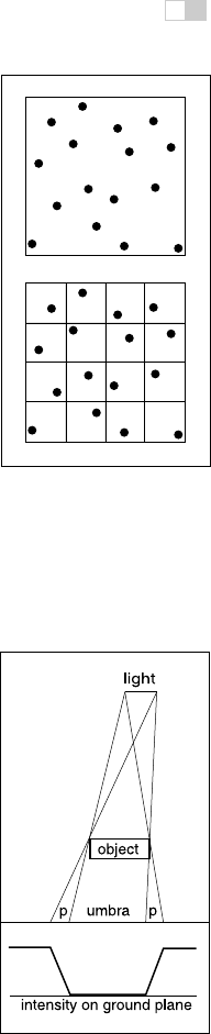
in 2D in Figure 13.12. The region where the light is entirely invisible is called
the umbra. The partially visible region is called the penumbra. There is not a
commonly used term for the region not in shadow, but it is sometimes called the
anti-umbra.
The key to implementing soft shadows is to somehow account for the light
being an area rather than a point. An easy way to do this is to approximate the
light with a distributed set of N point lights each with one Nth of the intensity
of the base light. This concept is illustrated at the left of Figure 13.13 where nine
Figure 13.12. A
soft shadow has a gradual
transition from the unshad-
owed to shadowed region.
The transition zone is the
“penumbra” denoted by
p
in
the figure.
lights are used. You can do this in a standard ray tracer, and it is a common trick
to get soft shadows in an off-the-shelf renderer. There are two potential problems
with this technique. First, typically dozens of point lights are needed to achieve
visually smooth results, which slows down the program a great deal. The second
problem is that the shadows have sharp transitions inside the penumbra.
Distribution ray tracing introduces a small change in the shadowing code.
Instead of representing the area light at a discrete number of point sources, we
represent it as an infinite number and choose one at random for each viewing ray.
i
i
i
i
i
i
i
i
312 13. More Ray Tracing
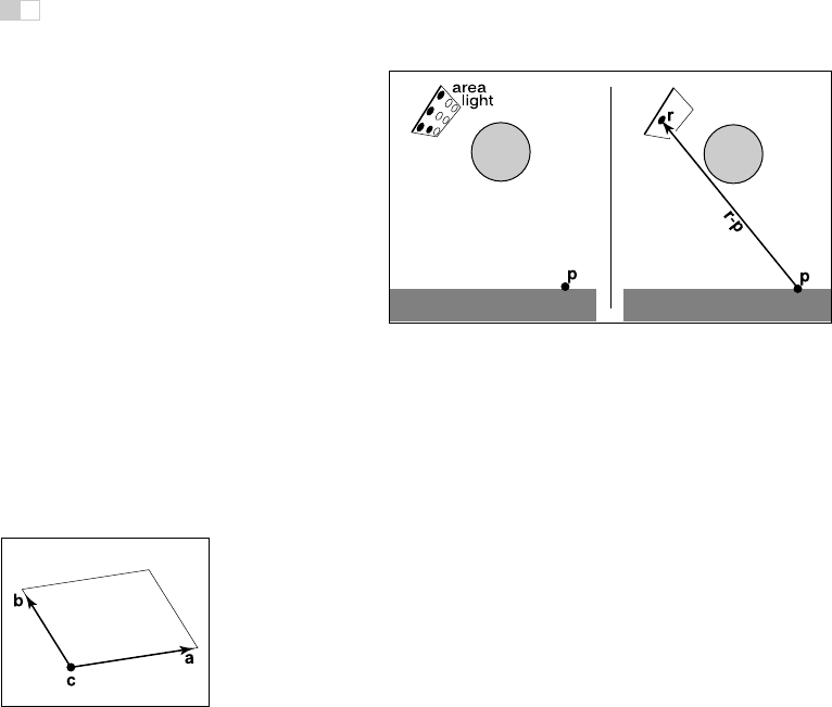
Figure 13.13. Left: an area light can be approximated by some number of point lights; four
of the nine points are visible to p so it is in the penumbra. Right: a random point on the light
is chosen for the shadow ray, and it has some chance of hitting the light or not.
This amounts to choosing a random point on the light for any surface point being
lit as is shown at the right of Figure 13.13.
If the light is a parallelogram specified by a corner point c and two edge
vectors a and b (Figure 13.14), then choosing a random point r is straightforward:
r = c + ξ
1
a + ξ
2
b,
where ξ
1
and ξ
2
are uniform random numbers in the range [0, 1).
We then send a shadow ray to this point as shown at the right in Figure 13.13.
Note that the direction of this ray is not unit length, which may require some
modification to your basic ray tracer depending upon its assumptions.
Figure 13.14. The geom-
etry of a parallelogram light
specified by a corner point
and two edge vectors.
We would really like to jitter points on the light. However, it can be dangerous
to implement this without some thought. We would not want to always have the
ray in the upper left-hand corner of the pixel generate a shadow ray to the upper
left-hand corner of the light. Instead we would like to scramble the samples, such
that the pixel samples and the light samples are each themselves jittered, but so
that there is no correlation between pixel samples and light samples. A good way
to accomplish this is to generate two distinct sets of n
2
jittered samples and pass
samples into the light source routine:
for each pixel (i, j) do
c =0
generate N = n
2
jittered 2D points and store in array r[]
generate N = n
2
jittered 2D points and store in array s[]
shuffle the points in array s[]
for p =0to N − 1 do
c = c + ray-color(i + r[p].x(), j + r[p].y(),s[p])
c
ij
= c/N
..................Content has been hidden....................
You can't read the all page of ebook, please click here login for view all page.