

i
i
i
i
i
i
i
i
428 17. Computer Animation
Each of the skeleton’s joints acts as a parent for the hierarchy below it. The
root represents the whole character and is positioned directly in the world coor-
dinate system. If a local transformation matrix which relates a joint to its parent
in the hierarchy is available, one can obtain a transformation which relates local
space of any joint to the world system (i.e., the system of the root) by simply con-
catenating transformations along the path from the root to the joint. To evaluate
the whole skeleton (i.e., find position and orientation of all joints), a depth-first
traversal of the complete tree of joints is performed. A transformation stack is a
natural data structure to help with this task. While traversing down the tree, the
current composite matrix is pushed on the stack and new one is created by mul-
tiplying the current matrix with the one stored at the joint. When backtracking
to the parent, this extra transformation should be undone before another branch is
visited; this is easily done by simply popping the stack. Although this general and
simple technique for evaluating hierarchies is used throughout computer graphics,
in animation (and robotics) it is given a special name—forward kinematics (FK).
While general representations for all transformations can be used, it is common to
use specialized sets of parameters, such as link lengths or joint angles, to specify
skeletons. To animate with forward kinematics, rotational parameters of all joints
are manipulated directly. The technique also allows the animator to change the
distance between joints (link lengths), but one should be aware that this corre-
sponds to limb stretching and can often look rather unnatural.
Forward kinematics requires the user to set parameters for all joints involved
in the motion (Figure 17.16 (top)). Most of these joints, however, belong to in-
Original
After hip rotation
After knee rotation
Effector motion
hip and knee joint angles
computed automatically
IK solver connection
Figure 17.16. Forward kinematics (top) requires the animator to put all joints into correct
position. In inverse kinematic (bottom), parameters of some internal joints are computed
based on desired end effector motion.
i
i
i
i
i
i
i
i
17.4. Character Animation 429
ternal nodes of the hierarchy, and their motion is typically not something the
animator wants to worry about. In most situations, the animator just wants them
to move naturally “on their own,” and one is much more interested in specify-
ing the behavior of the end point of a joint chain, which typically corresponds to
something performing a specific action, such as an ankle or a tip of a finger. The
animator would rather have parameters of all internal joints be determined from
the motion of the end effector automatically by the system. Inverse kinematics
(IK) allows us to do just that (see Figure 17.16 (bottom)).
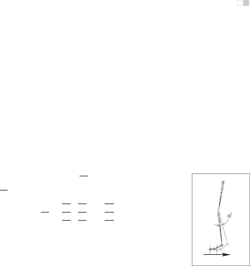
Let x be the position of the end effector and α be the vector of parameters
needed to specify all internal joints along the chain from the root to the final joint.
Sometimes the orientation of the final joint is also directly set by the animator, in
which case we assume that the corresponding variables are included in the vector
x. For simplicity, however, we will write all specific expressions for the vector:
x =(x
1
,x
2
,x
3
)
T
.
Since each of the variables in x is a function of α, it can be written as a vector
equation x = F(α). If we change the internal joint parameters by a small amount
δα, a resulting change δx in the position of the end effector can be approximately
written as
δx =
∂F
∂α
δα, (17.1)
where
∂F
∂α
is the matrix of partial derivatives called the Jacobian:
∂F
∂α
=
⎡
⎢
⎣
∂f
1
∂α
1
∂f
1
∂α
2
...
∂f
1
∂α
n
∂f
2
∂α
1
∂f
2
∂α
2
...
∂f
2
∂α
n
∂f
3
∂α
1
∂f
3
∂α
2
...
∂f
3
∂α
n
⎤
⎥
⎦
.
At each moment in time, we know the desired position of the end effector (set by
the animator) and, of course, the effector’s current position. Subtracting the two,
we will get the desired adjustment δx. Elements of the Jacobian matrix are related
to changes in a coordinate of the end effector when a particular internal parameter
is changed while others remain fixed (see Figure 17.17). These elements can
X
X
knee
Δ
Δ
Figure 17.17. Partial
derivative ∂
x
/∂α
knee
is
given by the limit of
Δ
x
/Δα
knee
. Effector dis-
placement is computed
while all joints, except the
knee, are kept fixed.
be computed for any given skeleton configuration using geometric relationships.
The only remaining unknowns in the system of equations(17.1) are the changes in
internal parameters α. Once we solve for them, we updateα = α+δα which gives
all the necessary information for the FK procedure to reposition the skeleton.
Unfortunately, the system (17.1) can not usually be solved analytically and,
moreover, it is in most cases underconstrained, i.e., the number of unknown inter-
nal joint parameters α exceeds the number of variables in vector x. This means
that different motions of the skeleton can result in the same motion of the end

i
i
i
i
i
i
i
i
430 17. Computer Animation
effector. Some examples are shown on Figure 17.18. Many ways of obtaining
specific solution for such systems are available, including those taking into ac-
count natural constraints needed for some real-life joints (bending a knee only in
one direction, for example). One should also remember that the computed Jaco-
bian matrix is valid only for one specificconfiguration, and it has to be updated as
the skeleton moves. The complete IK framework is presented in Figure 17.19. Of
IK root
effector
position
Figure 17.18. Mul-
tiple configurations of in-
ternal joints can result in
the same effector position.
(Top) disjoint “flipped” solu-
tions; (bottom) a continuum
of solutions.
course, the root joint for IK does not have to be the root of the whole hierarchy,
and multiple IK solvers can be applied to independent parts of the skeleton. For
example, one can use separate solvers for right and left feet and yet another one
to help animate grasping with the right hand, each with its own root.
Old skeleton configuration
Update constraints
new values for internal joint parameters
replace old skeleton
configuration with the new one
YES, done
NO
new skeleton configuration
solve equation 1.1
Compute the Jacobian and
desired effector motion
apply forward kinematic to reposition skeleton
Effector at desired position ?
Figure 17.19. A diagram of the inverse kinematic
algorithm.
A combination of FK
and IK approaches is typ-
ically used to animate the
skeleton. Many com-
mon motions (walking or
running cycles, grasping,
reaching, etc.) exhibit well-
known patterns of mutual
joint motion making it pos-
sible to quickly create nat-
urally looking motion or
even use a library of such
“clips.” The animator then
adjusts this generic result
according to the physical
parameters of the character
andalsotogiveitmorein-
dividuality.
When a skeleton changes its position, it acts as a special type of deformer
applied to the skin of the character. The motion is transferred to this surface by
Figure 17.20. Top:
Rigid skinning assigns skin
vertices to a specific joint.
Those belonging to the el-
bow joint are shown in
black; Bottom: Soft skin-
ning can blend the in-
fluence of several joints.
Weights for the elbow joint
are shown (lighter = greater
weight). Note smoother
skin deformation of the in-
ner part of the skin near the
joint.
assigning each skin vertex one (rigid skinning)ormore(smooth skinning) joints
as drivers (see Figure 17.20). In the first case, a skin vertex is simply frozen
into the local space of the corresponding joint, which can be the one nearest in
space or one chosen directly by the user. The vertex then repeats whatever mo-
tion this joint experiences, and its position in world coordinates is determined by
standard FK procedure. Although it is simple, rigid skinning makes it difficult
to obtain sufficiently smooth skin deformation in areas near the joints or also for
more subtle effects resembling breathing or muscle action. Additional specialized
deformers called flexors can be used for this purpose. In smooth skinning, several
joints can influence a skin vertex according to some weight assigned by the ani-
i
i
i
i
i
i
i
i
17.4. Character Animation 431
mator, providing more detailed control over the results. Displacement vectors, d
i
,
suggested by different joints affecting a given skin vertex (each again computed
with standard FK) are averaged according to their weights w
i
to compute the fi-
nal displacement of the vertex d =
(
w
i
d
i
. Normalized weights (
(
w
i
=1)
are the most common but not fundamentally necessary. Setting smooth skinning
weights to achieve the desired effect is not easy and requires significant skill from
the animator.
17.4.1 Facial Animation
Skeletons are well suited for creating most motions of a character’s body, but they
are not very convenient for realistic facial animation. The reason is that the skin
of a human face is moved by muscles directly attached to it contrary to other parts
of the body where the primary objective of the muscles is to move the bones of
the skeleton and any skin deformation is a secondary outcome. The result of this
facial anatomical arrangement is a very rich set of dynamic facial expressions
humans use as one of the main instruments of communication. We are all very
well trained to recognize such facial variations and can easily notice any unnatural
appearance. This not only puts special demands on the animator but also requires
a high-resolution geometric model of the face and, if photorealism is desired,
accurate skin reflection properties and textures.
While it is possible to set key poses of the face vertex-by-vertex and inter-
polate between them or directly simulate the behavior of the underlying muscle
structure using physics-based techniques (see Section 17.5 below), more special-
ized high-level approaches also exist. The static shape of a specific face can be
characterized by a relatively small set of so-called conformational parameters
(overall scale, distance from the eye to the forehead, length of the nose, width of
the jaws, etc.) which are used to morph a generic face model into one with individ-
ual features. An additional set of expressive parameters can be used to describe
the dynamic shape of the face for animation. Examples include rigid rotation of
the head, how wide the eyes are open, movement of some feature point from its
static position, etc. These are chosen so that most of the interesting expressions
can be obtained through some combination of parameter adjustments, therefore,
allowing a face to be animated via standard keyframing. To achieve a higher level
of control, one can use expressive parameters to create a set of expressions corre-
sponding to common emotions (neutral, sadness, happiness, anger, surprise, etc.)
and then blend these key poses to obtain a “slightly sad” or “angrily surprised”
face. Similar techniques can be used to perform lip-synch animation, but key
poses in this case correspond to different phonemes. Instead of using a sequence
i
i
i
i
i
i
i
i
432 17. Computer Animation
of static expressions to describe a dynamic one, the Facial Action Coding Sys-
tem (FACS) (Eckman & Friesen, 1978) decomposes dynamic facial expressions
directly into a sum of elementary motions called action units (AUs). The set of
AUs is based on extensive psychological research and includes such movements
as raising the inner brow, wrinkling the nose, stretching lips, etc. Combining AUs
can be used to synthesize a necessary expression.
17.4.2 Motion Capture
Even with the help of the techniques described above, creating realistic-looking
character animation from scratch remains a daunting task. It is therefore only
natural that much attention is directed towards techniques which record an actor’s
motion in the real world and then apply it to computer-generated characters. Two
main classes of such motion capture (MC) techniques exist: electromagnetic and
optical.
In electromagnetic motion capture, an electromagnetic sensor directly mea-
sures its position (and possibly orientation) in 3D often providing the captured
results in real time. Disadvantages of this technique include significant equip-
ment cost, possible interference from nearby metal objects, and noticeable size
of sensors and batteries which can be an obstacle in performing high-amplitude
motions. In optical MC, small colored markers are used instead of active sensors
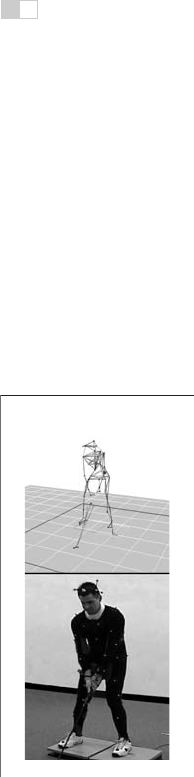
making it a much less intrusive procedure. Figure 17.21 shows the operation of
such a system. In the most basic arrangement, the motion is recorded by two cali-
brated video cameras, and simple triangulation is used to extract the marker’s 3D
position. More advanced computer vision algorithms used for accurate tracking
of multiple markers from video are computationally expensive, so, in most cases,
such processing is done offline. Optical tracking is generally less robust than
Figure 17.21. Optical
motion capture: markers
attached to a performer’s
body allow skeletal motion
to be extracted.
Image
courtesy of Motion Analysis
Corp.
electromagnetic. Occlusion of a given marker in some frames, possible misiden-
tification of markers, and noise in images are just a few of the common problem
which have to be addressed. Introducing more cameras observing the motion from
different directions improves both accuracy and robustness, but this approach is
more expensive and it takes longer to process such data. Optical MC becomes
more attractive as available computational power increases and better computer
vision algorithms are developed. Because of low impact nature of markers, opti-
cal methods are suitable for delicate facial motion capture and can also be used
with objects other than humans—for example, animals or even tree branches in
the wind.
With several sensors or markers attached to a performer’s body, a set of time-
dependant 3D positions of some collection of points can be recorded. These track-
..................Content has been hidden....................
You can't read the all page of ebook, please click here login for view all page.