
i
i
i
i
i
i
i
i
6.1. 2D Linear Transformations 121
matrix, with the rotations and scales already mixed together. This kind of manip-
ulation can be achieved if the matrix can be computationallydisassembled into the
desired pieces, the pieces adjusted, and the matrix reassembled by multiplying the
pieces together again.
It turns out that this decomposition, or factorization, is possible, regardless of
the entries in the matrix—and this fact provides a fruitful way of thinking about
transformations and what they do to geometry that is transformed by them.
Symmetric Eigenvalue Decomposition
Let’s start with symmetric matrices. Recall from Section 5.4 that a symmetric ma-
trix can always be taken apart using the eigenvalue decomposition into a product
of the form
A = RSR
T
where R is an orthogonal matrix and S is a diagonal matrix; we will call the
columns of R (the eigenvectors) by the names v
1
and v
2
, and we’ll call the diag-
onal entries of S (the eigenvalues) by the names λ
1
and λ
2
.
In geometric terms we can now recognize R as a rotation and S as a scale, so
this is just a multi-step geometric transformation (Figure 6.13):
1. Rotate v
1
and v
2
to the x-andy-axes (the transform by R
T
).
2. Scale in x and y by (λ
1
,λ
2
) (the transform by S).
3. Rotate the x-andy-axes back to v
1
and v
2
(the transform by R).
If you like to count di-
mensions: a symmetric 2
× 2 matrix has 3 de-
grees of freedom, and the
eigenvalue decomposition
rewrites them as a rotation
angle and two scale factors.
Looking at the effect of these three transforms together, we can see that they have
the effect of a nonuniform scale along a pair of axes. As with an axis-aligned
scale, the axes are perpendicular, but they aren’t the coordinate axes; instead they
R
T
v
2
v
1
σ
2
v
2
σ
1
v
1
SR
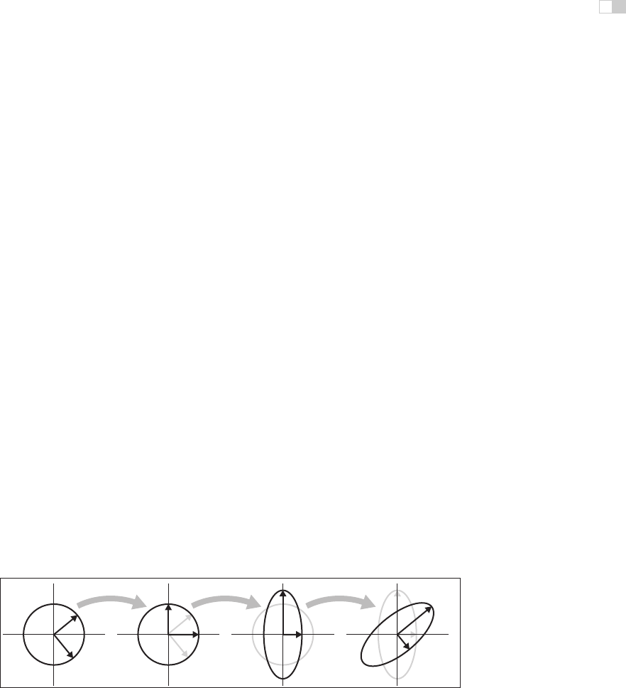
Figure 6.13. What happens when the unit circle is transformed by an arbitrary symmetric
matrix A, also known as a non–axis-aligned, nonuniform scale. The two perpendicular vec-
tors v
1
and v
2
, which are the eigenvectors of A, remain fixed in direction but get scaled. In
terms of elementary transformations, this can be seen as first rotating the eigenvectors to
the canonical basis, doing an axis-aligned scale, and then rotating the canonical basis back
to the eigenvectors.

i
i
i
i
i
i
i
i
122 6. Transformation Matrices
Figure 6.14. A symmetric matrix is always a scale along some axis. In this case it is along
the φ = 31.7
◦
direction which means the real eigenvector for this matrix is in that direction.
are the eigenvectors of A. This tells us something about what it means to be a
symmetric matrix: symmetric matrices are just scaling operations—albeit poten-
tially nonuniform and non–axis-aligned ones.
Example. Recall the example from Section 5.4:
21
11
= R
λ
1
0
0 λ
2
R
T
=
0.8507 −0.5257
0.5257 0.8507
2.618 0
00.382
0.8507 0.5257
−0.5257 0.8507
= rotate (31.7
◦
) scale (2.618, 0.382) rotate (−31.7
◦
).
The matrix above, then, according to its eigenvalue decomposition, scales in a
direction 31.7
◦
counterclockwise from three o’clock (the x-axis). This is a touch
before 2 p.m. on the clockface as is confirmed by Figure 6.14.
We can also reverse the diagonalization process; to scale by (λ
1
,λ
2
) with the
first scaling direction an angle φ clockwise from the x-axis, we have
cos φ sin φ
−sin φ cos φ
λ
1
0
0 λ
2
cos φ −sin φ
sin φ cos φ
=
λ
1
cos
2
φ + λ
2
sin
2
φ (λ
2
− λ
1
)cosφ sin φ
(λ
2
− λ
1
)cosφ sin φλ
2
cos
2
φ + λ
1
sin
2
φ
.
We should take heart that this is a symmetric matrix as we know must be true
since we constructed it from a symmetric eigenvalue decomposition.
i
i
i
i
i
i
i
i
6.1. 2D Linear Transformations 123
V
T
v
2
v
1
σ
2
u
2
σ
1
u
1
SU
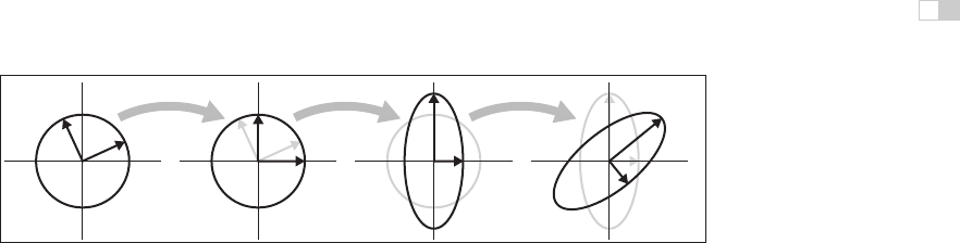
Figure 6.15. What happens when the unit circle is transformed by an arbitrary matrix A.
The two perpendicular vectors v
1
and v
2
, which are the right singular vectors of A, get scaled
and changed in direction to match the left singular vectors, u
1
and u
2
. In terms of elementary
transformations, this can be seen as first rotating the right singular vectors to the canonical
basis, doing an axis-aligned scale, and then rotating the canonical basis to the left singular
vectors.
Singular Value Decomposition
A very similar kind of decomposition can be done with non-symmetric matrices
as well: it’s the Singular Value Decomposition (SVD), also discussed in Sec-
tion 5.4.1. The difference is that the matrices on either side of the diagonal matrix
are no longer the same:
A = USV
T
The two orthogonal matrices that replace the single rotation R are called U and
V, and their columns are called u
i
(the left singular vectors)andv
i
(the right
singular vectors), respectively. In this context, the diagonal entries of S are called
singular values rather than eigenvalues. The geometric interpretation is very sim-
ilar to that of the symmetric eigenvalue decomposition (Figure 6.15):
1. Rotate v
1
and v
2
to the x-andy-axes (the transform by V
T
).
2. Scale in x and y by (σ
1
,σ
2
) (the transform by S).
3. Rotate the x-andy-axes to u
1
and u
2
(the transform by U).
For dimension counters: a
general 2
× 2 matrix has
4 degrees of freedom, and
the SVD rewrites them as
two rotation angles and two
scale factors. One more bit
is needed to keep track of
reflections, but that doesn’t
add a dimension.
The principal difference is between a single rotation and two different orthogonal
matrices. This difference causes another, less important, difference. Because the
SVD has different singular vectors on the two sides, there is no need for neg-
ative singular values: we can always flip the sign of a singular value, reverse
the direction of one of the associated singular vectors, and end up with the same
transformation again. For this reason, the SVD always produces a diagonal ma-
trix with all positive entries, but the matrices U and V are not guaranteed to be
rotations—they could include reflection as well. In geometric applications like
graphics this is an inconvenience, but a minor one: it is easy to differentiate ro-
tations from reflections by checking the determinant, which is +1 for rotations

i
i
i
i
i
i
i
i
124 6. Transformation Matrices
and −1 for reflections, and if rotations are desired, one of the singular values can
be negated, resulting in a rotation–scale–rotation sequence where the reflection is
rolled in with the scale, rather than with one of the rotations.
Example. The example used in Section 5.4.1 is in fact a shear matrix (Figure 6.12):
11
01
= R
2
σ
1
0
0 σ
2
R
1
=
0.8507 −0.5257
0.5257 0.8507
1.618 0
00.618
0.5257 0.8507
−0.8507 0.5257
= rotate (31.7
◦
) scale (1.618, 0.618) rotate (−58.3
◦
).
An immediate consequence of the existence of SVD is that all the 2D transforma-
tion matrices we have seen can be made from rotation matrices and scale matrices.
Shear matrices are a convenience, but they are not required for expressing trans-
formations.
In summary, every matrix can be decomposed via SVD into a rotation times
a scale times another rotation. Only symmetric matrices can be decomposed via
eigenvalue diagonalization into a rotation times a scale times the inverse-rotation,
and such matrices are a simple scale in an arbitrary direction. The SVD of a
symmetric matrix will yield the same triple product as eigenvalue decomposition
via a slightly more complex algebraic manipulation.
Paeth Decomposition of Rotations
Another decomposition uses shears to represent non-zero rotations (Paeth, 1990).
The following identity allows this:
cos φ −sin φ
sin φ cos φ
=
1
cos φ−1
sin φ
01
10
sin φ 1
1
cos φ−1
sin φ
01
.
For example, a rotation by π/4 (45 degrees) is (see Figure 6.16)
rotate(
π
4
)=
11−
√
2
01
10
√
2
2
1
11−
√
2
01
. (6.2)
This particular transform is useful for raster rotation because shearing is a
very efficient raster operation for images; it introduces some jagginess, but will

i
i
i
i
i
i
i
i
6.2. 3D Linear Transformations 125
Figure 6.16. Any 2D rotation can be accomplished by three shears in sequence. In this
case a rotation by 45
◦
is decomposed as shown in Equation 6.2.
leave no holes. The key observation is that if we take a raster position (i, j) and
apply a horizontal shear to it, we get
1 s
01
i
j
=
i + sj
j
.
If we round sj to the nearest integer, this amounts to taking each row in the
image and moving it sideways by some amount—a different amount for each
row. Because it is the same displacement within a row, this allows us to rotate
with no gaps in the resulting image. A similar action works for a vertical shear.
Thus, we can implement a simple raster rotation easily.
6.2 3D Linear Transformations
The linear 3D transforms are an extension of the 2D transforms. For example, a
scale along Cartesian axes is
scale(s
x
,s
y
,s
z
)=
⎡
⎣
s
x
00
0 s
y
0
00s
z
⎤
⎦
. (6.3)
..................Content has been hidden....................
You can't read the all page of ebook, please click here login for view all page.