
i
i
i
i
i
i
i
i
390 16. Implicit Modeling
with distance fields started with Ricci (Ricci, 1973); R-functions (Rvachev, 1963)
were first applied to shape modeling more than 20 years later (see (Shapiro, 1994)
and (A. Pasko et al., 1995)).
An R-function or Rvachev function is a function whose sign can change if
and only if the sign of one of its arguments changes; that is, its sign is determined
solely by its arguments. R-functions provide a robust theoretical framework for
boolean composition of real functions, permitting the construction of C
n
CSG
operators (Shapiro, 1988). These CSG operators can be used to create blending
operators simply by adding a fixed offset to the result (A. Pasko et al., 1995).
Although these blending functions are no longer technically R-functions, they
have most of the desirable properties and can be mixed freely with R-functions
to create complex hierarchical models (Shapiro, 1988). These R-function-based
blending and CSG operators are referred to as R-operators (see Section 16.4).
The Hyperfun system (Adzhiev et al., 1999) is based on F-reps (function repre-
sentation), another name for an implicit surface. The system uses a procedural
C-like language to describe many types of implicit surfaces.
16.1.3 Level Sets
It is useful to represent an implicit field discretely via a regular grid (Barthe et al.,
2002) or an adaptive grid (Frisken et al., 2000). This is exactly what the polygo-
nization algorithm does in the case of level sets; moreover, the grid can be used
for various other purposes beside building polygons. Discrete representations of
f are commonly obtained by sampling a continuous function at regular intervals.
For example, the sampled function may be defined by other volume model repre-
sentations (V. V. Savchenko et al., 1998). The data may also be a physical object
sampled using three-dimensional imaging techniques. Discrete volume data has
most often been used in conjunction with the level sets method (Osher & Sethian,
1988), which defines a means for dynamically modifying the data structure using
curvature-dependent speed functions. Interactive modeling environments based
on level sets have been defined (Museth et al., 2002), although level sets are only
one method employing a discrete representation of the implicit field. Methods
for interactively defining discrete representations using standard implicit surfaces
techniques have also been explored (Baerentzen & Christensen, 2002).
A key advantage to employing a discrete data structure is its ability to act as a
unifying approach for all of the various volume models defined by potential fields
(discrete or not) (V. V. Savchenko et al., 1998). The conversion of any continuous
function to a discrete representation introduces the problem of how to reconstruct
a continuous function, needed for the combined purposes of additional modeling

i
i
i
i
i
i
i
i
16.1. Implicit Functions, Skeletal Primitives and Summation Blending 391
operations and visualization of the resulting potential field. A well knownsolution
to this problem is to apply a filter g using the convolution operator (see Chapter 9).
The choice of a filter is guided by the desired properties of the reconstruction, and
many filters have been explored (Marschner & Lobb, 1994). The salient point is
that there is typically a trade-off between the efficiency of the chosen filter and
the smoothness of the resulting reconstruction; see also Section 16.9.
To be interactive, a discrete system must restrict the size of the grid relative
to the available computing power. This, in turn, limits the ability of the mod-
eler to include high-frequency details. Additionally, the smoothing triquadratic
filter makes it impossible to include sharp edges should they be desired. A par-
tial solution to this problem is the use of adaptive grids, although with any dis-
crete representation there will be limitations. A discrete grid is used in (Schmidt,
Wyvill, & Galin, 2005) to act as a cache representing a BlobTree node. The grid in
this work is used for fast prototyping and uses trilinear interpolation for position
and the slower, more accurate triquadratic interpolation to calculate gradient val-
ues, because the eye is more discerning in observing gradient errors than position
errors.
16.1.4 Variational Implicit Surfaces
It is often required to convert sampled data to an implicit representation. Varia-
tional implicit surfaces interpolate or approximate a set of points using a weighted
sum of globally-supported basis functions (V. Savchenko et al., 1995; Turk &
O’Brien, 1999; J. C. Carr et al., 2001; Turk & O’Brien, 2002). These radially
symmetric basis functions are applied at each sample point. The continuity of
such a surface depends on the choice of basis function. The C
2
thin-plate spline
is most commonly used (Turk & O’Brien, 2002; J. C. Carr et al., 2001). Like
Blinn’s exponential function (see Figure 16.2), this function is unbounded as is
the resulting variational implicit surface.
If the fieldisisgloballyC
2
, creases cannot be defined;
2
however, anisotropic
basis functions can be used to produce fields which change more rapidly and may
appear to have creases (Dinh et al., 2001). At the appropriate scale, the surface
is still smooth. The smooth field implies that self-intersections do not occur, and
hence volumes are always well-defined. The thin-plate spline guarantees that
global curvature is minimized (Duchon,1977). Variational interpolation has many
properties which are desirable for 3D modeling, however controlling the resulting
surfaces can be difficult.
2
Except see Section 15.2.
i
i
i
i
i
i
i
i
392 16. Implicit Modeling
Variational implicit surfaces can also be based on compactly-supported radial
basis functions (CS-RBFs) to reduce the computational cost of variational inter-
polation techniques (Morse et al., 2001). Each CS-RBF only influences a local
region, so computing f(p) requires only evaluation of basis functions within some
small neighborhood of p. As with the globally-supported counterpart, the result-
ing field is C
k
, creases are not supported, and self-intersections cannot occur.
3
The local support of each basis function results in a bounded global field. This
also guarantees that additional iso-contours will be present, as noted by various
researchers (Ohtake et al., 2003; Reuter, 2003).
16.1.5 Convolution Surfaces
Convolution surfaces, introduced by Bloomenthal and Shoemake (Bloomenthal
& Shoemake, 1991) are produced by convolving a geometric skeleton S with a
kernel function h. Hence, the value at any position in space is defined by an
integral over the skeleton:
f(p)=
S
g(r) h(p − r) dr.
Any finitely-supported function can be used as h; see (Sherstyuk, 1999) for a
detailed analysis of different kernels.
Like skeletal primitives, convolution surfaces have bounded fields. Blinn’s
“blobby molecules” is the simplest form of a convolutionsurface (J. Blinn, 1982);
in this case, the skeleton consists of points only. This idea was extended by
Bloomenthal to include line, arc, triangle, and polygon skeletons (Bloomenthal
& Shoemake, 1991). These represent 1D and 2D primitives; 3D primitives were
later described by Bloomenthal (Bloomenthal, 1995).
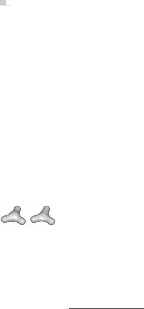
Figure 16.4. Two blended
cylinders. Left: summa-
tion blend; right: convolu-
tion surface with barely dis-
cernible bulge (Bloomen-
thal, 1997).
Image courtesy
Erwin DeGroot
.
Combination of convolution surfaces is defined by composition of the under-
lying geometric skeletons and has the advantage of eliminating the bulges that
tend to occur when composing multiple skeletal primitives with additive blend-
ing. The surface resulting from convolution of the combined skeleton does not
have bulges, as in Figure 16.4, and the field is continuous even if the combined
skeleton is non-convex. Convolution surfaces are offset a fixed distance from
convex portions of a skeleton, but produce a fillet along concave portions of a
skeleton.
An exampleof skeletal elements convolved to build a complex model is shown
in Figure 16.5. The hand model contains fourteen primitives.
3
Note, k>0 depending on the RBF (see Section 15.2).

i
i
i
i
i
i
i
i
16.1. Implicit Functions, Skeletal Primitives and Summation Blending 393
Figure 16.5. Skeletal elements convolved to build a hand model.
Image courtesy Jules
Bloomenthal.
16.1.6 Defining Skeletal Primitives
As we will see in the following sections rendering the implicit models requires
finding the field value and gradient for a large number of points. We need the
distance to supply to Equation (16.2) and the gradient is useful for root finding as
well as lighting calculations. Supplying the distance to the fall-off filter functions
of Figure 16.2 is a matter of calculating the nearest distance to the skeletal primi-
tive, simple for point primitives but a little trickier for more complex geometrical
shapes. A line segment primitive (AB) can be defined as a cylinder around a line
with hemispherical end caps (see Figure 16.6). Point P
0
lies on the surface where
Figure 16.6. Line primi-
tive
ab
and example points
p
0
,
p
1
,
p
2
showing distance
calculation.
f(P
0
)=isoand f(P
1
)=0since it lies outside of the influence of the line primi-
tive. The distance from some P
i
to the line is found by simply projecting onto the
line AB and calculating the perpendicular distance, e.g., |CP
0
|; this can be found
from AC,sinceA, P
0
, and B, are all known:
AC =
AB
AP
0
·
AB
AB
2
.
In Figure 16.6 the field value of P
2
> 0,sinceP
2
is in the hemispherical end-
cap, which can be checked separately. Variations of this idea can define primitives

i
i
i
i
i
i
i
i
394 16. Implicit Modeling
with endcaps of different radii producing interesting cone shapes. An example is
shown in Figure 16.7.
Figure 16.7. Cylin-
der primitive blended with a
sphere.
Image courtesy Er-
win DeGroot
.
A great variety of geometrical skeletons have been described, and, in princi-
ple, it is simply a matter of defining the distance to the skeleton from some point p
and also the gradient at p. For example, an offset surface of a triangle can be de-
fined from the vertices of the triangle and a radius r. A simple way to implement
this is to use line segment primitives to describe bounding cylinders connecting
the vertices (radius r). The distance from a point q within the triangle that does
not fall within the bounding fields of one of the line segment primitives is returned
as the perpendicular distance to the plane of the triangle. Other examples include
an implicit disk, defined by a circle and a thickness parameter, a torus also defined
by a circle and the radius of the cross section (or inner and outer circle radii), a
circular cone from a disk and a height, a cube with rounded corners, etc. (see
Figure 16.8).
16.2 Rendering
Modeling methods, such as parametric surfaces, lend themselves to visualization,
since it is easy to iterate over points on the surface that can be found directly from
the defining equations; for example (x, y)=(cosθ, sin θ),θ∈ [0, 2π) produces
a circle.
Figure 16.8. Implicit
models from various skele-
tal primitives.
Image cour-
tesy Erwin DeGroot
.
There are two techniques that are commonly used to render implicit surfaces:
ray tracing and surface tiling. In practice, a designer wants to visualize an implicit
surface model quickly, sacrificing quality for speed for interaction purposes. Pro-
totyping algorithms have been concerned with producing a polygon mesh that can
be rendered in real time on modern workstations. Finding the polygonal mesh
which best approximates the desired surface is referred to as polygonization or
surface tiling. For animation or for a final visualization, where quality is pre-
ferred over speed, ray tracing implicit surfaces directly without first polygonizing
produces excellent results.
Figure 16.9. Aray-traced
dinosaur model showing
the underlying skeletal
primitives.
Image courtesy
Erwin DeGroot
.
As previously mentioned, finding an implicit surface requires searching
through space to find the points that satisfy, f(p)=0. There are two main ap-
proaches to executing such a search: space partitioning—partitioning space into
manageable units such as cubes, and non-space partitioning, e.g., marching trian-
gles (Hartmann, 1998; Akkouche & Galin, 2001) and the shrinkwrap algorithm
(Overveld & Wyvill, 2004).
In this chapter we describe the original space partitioning algorithm and leave
it to the reader to explore the more advanced methods. This algorithm together
..................Content has been hidden....................
You can't read the all page of ebook, please click here login for view all page.