i
i
i
i
i
i
i
i
8
The Graphics Pipeline
The previous several chapters have established the mathematical scaffolding we
need to look at the second major approach to rendering: drawing objects one by
one onto the screen, or object-order rendering. Unlike in ray tracing, where we
consider each pixel in turn and find the objects that influence its color, we’ll now
instead consider each geometric object in turn and find the pixels that it could have
an effect on. The process of finding all the pixels in an image that are occupied by
Any graphics system has
one or more types of “prim-
itive object” that it can han-
dle directly, and more com-
plex objects are converted
into these “primitives.” Tri-
angles are the most often
used primitive.
a geometric primitive is called rasterization, so object-order rendering can also
be called rendering by rasterization. The sequence of operations that is required,
Rasterization-based sys-
tems are also called
scanline renderers
.
starting with objects and ending by updating pixels in the image, is known as the
graphics pipeline.
Object-order rendering has enjoyed great success because of its efficiency.
For large scenes, management of data access patterns is crucial to performance,
and making a single pass over the scene visiting each bit of geometry once has
significant advantages over repeatedly searching the scene to retrieve the objects
required to shade each pixel.
The title of this chapter suggests that there is only one way to do object-
order rendering. Of course this isn’t true—two quite different examples of graph-
ics pipelines with very different goals are the hardware pipelines used to sup-
port interactive rendering via APIs like OpenGL and Direct3D and the software
pipelines used in film production, supporting APIs like RenderMan. Hardware
pipelines must run fast enough to react in real time for games, visualizations,
and user interfaces. Production pipelines must render the highest quality anima-
tion and visual effects possible and scale to enormous scenes, but may take much
161

i
i
i
i
i
i
i
i
162 8. The Graphics Pipeline
more time to do so. Despite the different design decisions resulting from these
divergent goals, a remarkable amount is shared among most, if not all, pipelines,
and this chapter attempts to focus on these common fundamentals, erring on the
side of following the hardware pipelines more closely.
The work that needs to be done in object-order rendering can be organized
into the task of rasterization itself, the operations that are done to geometry be-
fore rasterization, and the operations that are done to pixels after rasterization.
The most common geometric operation is applying matrix transformations, as
discussed in the previous two chapters, to map the points that define the geometry
from object space to screen space, so that the input to the rasterizer is expressed
in pixel coordinates, or screen space. The most common pixelwise operation is
hidden surface removal which arranges for surfaces closer to the viewer to appear
in front of surfaces farther from the viewer. Many other operations also can be in-
cluded at each stage, thereby achieving a wide range of different rendering effects
using the same general process.
For the purposes of this chapter we’ll discuss the graphics pipeline in terms of
four stages (Figure 8.1). Geometric objects are fed into the pipeline from an inter-
DISPLAY
BLENDING
FRAMEBUFFER IMAGE
FRAGMENTS
TRANSFORMED GEOMETRY
COMMAND STREAM
FRAGMENT PROCESSING
RASTERIZATION
VERTEX PROCESSING
APPLICATION
Figure 8.1. The stages of
a graphics pipeline.
active application or from a scene description file, and they are always described
by sets of vertices. The vertices are operated on in the vertex-processing stage,
then the primitives using those vertices are sent to the rasterization stage.The
rasterizer breaks each primitive into a number of fragments, one for each pixel
covered by the primitive. The fragments are processed in the fragment processing
stage, and then the various fragments corresponding to each pixel are combined
in the fragment blending stage.
We’ll begin by discussing rasterization, then illustrate the purpose of the geo-
metric and pixel-wise stages by a series of examples.
8.1 Rasterization
Rasterization is the central operation in object-order graphics, and the rasterizer
is central to any graphics pipeline. For each primitive that comes in, the rasterizer
has two jobs: it enumerates the pixels that are covered by the primitive and it
interpolates values, called attributes, across the primitive—the purpose for these
attributes will be clear with later examples. The output of the rasterizer is a set of
fragments, one for each pixel covered by the primitive. Each fragment “lives” at
a particular pixel and carries its own set of attribute values.
In this chapter, we will present rasterization with a view toward using it to
render three-dimensionalscenes. The same rasterization methods are used to draw

i
i
i
i
i
i
i
i
8.1. Rasterization 163
lines and shapes in 2D as well—although it is becoming more and more common
to use the 3D graphics system “under the covers” to do all 2D drawing.
8.1.1 Line Drawing
Most graphics packages contain a line drawing command that takes two endpoints
in screen coodinates (see Figure 3.10) and draws a line between them. For exam-
ple, the call for endpoints (1,1) and (3,2) would turn on pixels (1,1) and (3,2) and
fill in one pixel between them. For general screen coordinate endpoints (x
0
,y
0
)
and (x
1
,y
1
), the routine should draw some “reasonable” set of pixels that approx-
imate a line between them. Drawing such lines is based on line equations, and we
Even though we often use
integer-valued endpoints
for examples, it’s impor-
tant to properly support
arbitrary endpoints.
have two types of equations to choose from: implicit and parametric. This section
describes the approach using implicit lines.
Line Drawing Using Implicit Line Equations
The most common way to draw lines using implicit equations is the midpoint al-
gorithm (Pitteway (1967); van Aken and Novak (1985)). The midpoint algorithm
ends up drawing the same lines as the Bresenham algorithm (Bresenham, 1965)
but it is somewhat more straightforward.
The first thing to do is find the implicit equation for the line as discussed in
Section 2.5.2:
f(x, y) ≡ (y
0
− y
1
)x +(x
1
− x
0
)y + x
0
y
1
− x
1
y
0
=0. (8.1)
We assume that x
0
≤ x
1
. If that is not true, we swap the points so that it is true.
The slope m of the line is given by
m =
y
1
− y
0
x
1
− x
0
.
The following discussion assumes m ∈ (0, 1]. Analogous discussions can be
derived for m ∈ (−∞, −1], m ∈ (−1, 0],andm ∈ (1, ∞). The four cases cover
all possibilities.
For the case m ∈ (0, 1], there is more “run” than “rise,” i.e., the line is moving
faster in x than in y. IfwehaveanAPIwherethey-axis points downwards,
we might have a concern about whether this makes the process harder, but, in
fact, we can ignore that detail. We can ignore the geometric notions of “up”
and “down,” because the algebra is exactly the same for the two cases. Cautious
readers can confirm that the resulting algorithm works for the y-axis downwards
case. The key assumption of the midpoint algorithm is that we draw the thinnest

i
i
i
i
i
i
i
i
164 8. The Graphics Pipeline
line possible that has no gaps. A diagonal connection between two pixels is not
considered a gap.
As the line progresses from the left endpoint to the right, there are only two
possibilities: draw a pixel at the same height as the pixel drawn to its left, or draw
a pixel one higher. There will always be exactly one pixel in each column of pixels
Figure 8.2. Three
“reasonable” lines that go
seven pixels horizontally
and three pixels vertically.
between the endpoints. Zero would imply a gap, and two would be too thick a line.
There may be two pixels in the same row for the case we are considering; the line
is more horizontal than vertical so sometimes it will go right, and sometimes up.
This concept is shown in Figure 8.2, where three “reasonable” lines are shown,
each advancing more in the horizontal direction than in the vertical direction.
The midpoint algorithm for m ∈ (0, 1] first establishes the leftmost pixel and
the column number (x-value) of the rightmost pixel and then loops horizontally
establishing the row (y-value) of each pixel. The basic form of the algorithm is:
y = y
0
for x = x
0
to x
1
do
draw(x, y)
if (some condition) then
y = y +1
Note that x and y are integers. In words this says, “keep drawing pixels from left
to right and sometimes move upwards in the y-direction while doing so.” The key
is to establish efficient ways to make the decision in the if statement.
An effective way to make the choice is to look at the midpoint of the line
between the two potential pixel centers. More specifically, the pixel just drawn
is pixel (x, y) whose center in real screen coordinates is at (x, y). The candidate
pixels to be drawn to the right are pixels (x+1,y) and (x+1,y+1).The midpoint
between the centers of the two candidate pixels is (x +1,y +0.5). If the line
passes below this midpoint we draw the bottom pixel, and otherwise we draw the
top pixel (Figure 8.3).
To decide whether the line passes above or below (x+1,y+0.5),weevaluate
f(x, y +0.5) in Equation (8.1). Recall from Section 2.5.1 that f (x, y)=0for
points (x, y) on the line, f (x, y) > 0 for points on one side of the line, and
f(x, y) < 0 for
points on the other side of the line. Because −f(x, y)=0and
Figure 8.3. Top: the line
goes above the midpoint so
the top pixel is drawn. Bot-
tom: the line goes below
the midpoint so the bottom
pixel is drawn.
f(x, y)=0are both perfectly good equations for the line, it is not immediately
clear whether f(x, y) being positive indicates that (x, y) is above the line, or
whether it is below. However, we can figure it out; the key term in Equation (8.1)
is the y term (x
1
− x
0
)y. Note that (x
1
− x
0
) is definitely positive because
x
1
>x
0
. This means that as y increases, the term (x
1
−x
0
)y gets larger (i.e., more
positive or less negative). Thus, the case f(x, +∞) is definitely positive, and
definitely above the line, implying points above the line are all positive. Another

i
i
i
i
i
i
i
i
8.1. Rasterization 165
way to look at it is that the y component of the gradient vector is positive. So
above the line, where y can increase arbitrarily, f (x, y) must be positive. This
means we can make our code more specificbyfilling in the if statement:
if f(x +1,y+0.5) < 0 then
y = y +1
The above code will work nicely for lines of the appropriate slope (i.e., between
zero and one). The reader can work out the other three cases which differ only in
small details.
If greater efficiency is desired, using an incremental method can help. An
incremental method tries to make a loop more efficient by reusing computation
from the previous step. In the midpoint algorithm as presented, the main compu-
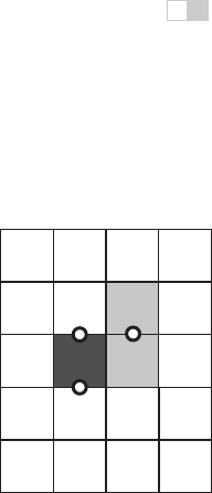
tation is the evaluation of f (x +1,y+0.5). Note that inside the loop, after the
first iteration, either we already evaluated f(x −1,y+0.5) or f(x − 1,y− 0.5)
(Figure 8.4). Note also this relationship:
Figure 8.4. When using
the decision point shown
between the two light gray
pixels, we just drew the
dark gray pixel, so we eval-
uated
f
at one of the two left
points shown.
f(x +1,y)=f (x, y)+(y
0
− y
1
)
f(x +1,y+1)=f(x, y)+(y
0
− y
1
)+(x
1
− x
0
).
This allows us to write an incremental version of the code:
y = y
0
d = f(x
0
+1,y
0
+0.5)
for x = x
0
to x
1
do
draw(x, y)
if d<0 then
y = y +1
d = d +(x
1
− x
0
)+(y
0
− y
1
)
else
d = d +(y
0
− y
1
)
This code should run faster since it has little extra setup cost compared to the
non-incremental version (that is not always true for incremental algorithms), but
it may accumulate more numeric error because the evaluation of f(x, y +0.5)
may be composed of many adds for long lines. However, given that lines are
rarely longer than a few thousand pixels, such an error is unlikely to be critical.
Slightly longer setup cost, but faster loop execution, can be achieved by storing
(x
1
−x
0
)+(y
0
−y
1
) and (y
0
−y
1
) as variables. We might hope a good compiler
would do that for us, but if the code is critical, it would be wise to examine the
results of compilation to make sure.
..................Content has been hidden....................
You can't read the all page of ebook, please click here login for view all page.
