
i
i
i
i
i
i
i
i
2.5. Curves and Surfaces 43
lies in the surface the vector q
also lies in the surface. Since it was obtained by
varying one argument of p, the vector q
is the partial derivative of p with respect
to u, which we’ll denote p
u
. A similar argument shows that the partial derivative
p
v
gives the tangent to the isoparametric curves for constant u, which is a second
tangent vector to the surface.
The derivative of p, then, gives two tangent vectors at any point on the sur-
face. The normal to the surface may be found by taking the cross product of
these vectors: since both are tangent to the surface, their cross product, which is
perpendicular to both tangents, is normal to the surface. The right-hand rule for
cross products provides a way to decide which side is the front, or outside, of the
surface; we will use the convention that the vector
n = p
u
× p
v
points toward the outside of the surface.
2.5.9 Summary of Curves and Surfaces
Implicit curves in 2D or surfaces in 3D are defined by scalar-valued functions of
two or three variables, f : R
2
→ R or f : R
3
→ R, and the surface consists of all
points where the function is zero:
S = {p |f (p)=0}.
Parametric curves in 2D or 3D are defined by vector-valued functions of one vari-
able, p : D ⊂ R → R
2
or p : D ⊂ R → R
3
, and the curve is swept out as t
varies over all of D:
S = {p(t) | t ∈ D }.
Parametric surfaces in 3D are defined by vector-valued functions of two variables,
p : D ⊂ R
2
→ R
3
, and the surface consists of the images of all points (u, v) in
the domain:
S = {p(t) | (u, v) ∈ D }.
For implicit curves and surfaces, the normal vector is given by the derivative
of f (the gradient), and the tangent vector (for a curve) or vectors (for a surface)
can be derived from the normal by constructing a basis.
For parametric curves and surfaces, the derivative of p gives the tangent vector
(for a curve) or vectors (for a surface), and the normal vector can be derived from
the tangents by constructing a basis.

i
i
i
i
i
i
i
i
44 2. Miscellaneous Math
2.6 Linear Interpolation
Perhaps the most common mathematical operation in graphics is linear interpo-
lation. We have already seen an example of linear interpolation of position to
form line segments in 2D and 3D, where two points a and b are associated with
a parameter t to form the line p =(1−t)a + tb.Thisisinterpolation because p
goes through a and b exactly at t =0and t =1.Itislinear interpolation because
the weighting terms t and 1 − t are linear polynomials of t.
Another common linear interpolation is among a set of positions on the x-
axis: x
0
, x
1
, ..., x
n
, and for each x
i
we have an associated height, y
i
.Wewantto
create a continuous function y = f(x) that interpolates these positions, so that f
goes through every data point, i.e., f(x
i
)=y
i
. For linear interpolation, the points
(x
i
,y
i
) are connected by straight line segments. It is natural to use parametric
line equations for these segments. The parameter t is just the fractional distance
between x
i
and x
i+1
:
f(x)=y
i
+
x − x
i
x
i+1
− x
i
(y
i+1
− y
i
). (2.27)
Because the weighting functions are linear polynomials of x, this is linear inter-
polation.
The two examples above have the common form of linear interpolation. We
create a variable t that varies from 0 to 1 as we move from data item A to data
item B. Intermediate values are just the function (1 − t)A + tB. Notice that
Equation (2.27) has this form with
t =
x − x
i
x
i+1
− x
i
.
2.7 Triangles
Triangles in both 2D and 3D are the fundamental modeling primitive in many
graphics programs. Often information such as color is tagged onto triangle ver-
tices, and this information is interpolated across the triangle. The coordinate sys-
tem that makes such interpolation straightforward is called barycentric coordi-
nates; we will develop these from scratch. We will also discuss 2D triangles,
which must be understood before we can draw their pictures on 2D screens.

i
i
i
i
i
i
i
i
2.7. Triangles 45
2.7.1 2D Triangles
If we have a 2D triangle defined by 2D points a, b,andc, we can first find its
area:
area =
1
2
x
b
− x
a
x
c
− x
a
y
b
− y
a
y
c
− y
a
=
1
2
(x
a
y
b
+ x
b
y
c
+ x
c
y
a
− x
a
y
c
− x
b
y
a
− x
c
y
b
) .
(2.28)
The derivation of this formula can be found in Section 5.3. This area will have a
positive sign if the points a, b,andc are in counterclockwise order and a negative
sign, otherwise.
Often in graphics, we wish to assign a property, such as color, at each trian-
gle vertex and smoothly interpolate the value of that property across the triangle.
There are a variety of ways to do this, but the simplest is to use barycentric co-
ordinates. One way to think of barycentric coordinates is as a non-orthogonal
coordinate system as was discussed briefly in Section 2.4.2. Such a coordinate
system is shown in Figure 2.36, where the coordinate origin is a and the vectors
from a to b and c are the basis vectors. With that origin and those basis vectors,
any point p can be written as
p = a + β(b − a)+γ(c −a). (2.29)
Figure 2.36. A 2D triangle with vertices a, b, c can be used to set up a non-orthogonal
coordinate system with origin a and basis vectors (b – a) and (c – a). A point is then
represented by an ordered pair (β, γ). For example, the point p = (2.0, 0.5), i.e., p = a
+2.0(b – a)+0.5(c – a).
i
i
i
i
i
i
i
i
46 2. Miscellaneous Math
Note that we can reorder the terms in Equation (2.29) to get
p =(1−β − γ)a + βb + γc.
Often people defineanewvariableα to improve the symmetry of the equations:
α ≡ 1 − β − γ,
which yields the equation
p(α, β, γ)=αa + βb + γc, (2.30)
with the constraint that
α + β + γ =1. (2.31)
Barycentric coordinates seem like an abstract and unintuitive construct at first,
but they turn out to be powerful and convenient. You may find it useful to think
of how street addresses would work in a city where there are two sets of parallel
streets, but where those sets are not at right angles. The natural system would
essentially be barycentric coordinates, and you would quickly get used to them.
Barycentric coordinates are defined for all points on the plane. A particularly nice
feature of barycentric coordinates is that a point p is inside the triangle formed by
a, b,andc if and only if
0 <α<1,
0 <β<1,
0 <γ<1.
If one of the coordinates is zero and the other two are between zero and one, then
you are on an edge. If two of the coordinates are zero, then the other is one,
and you are at a vertex. Another nice property of barycentric coordinates is that
Equation (2.30) in effect mixes the coordinates of the three vertices in a smooth
way. The same mixing coefficients (α, β, γ) can be used to mix other properties,
such as color, as we will see in the next chapter.
Given a point p, how do we compute its barycentric coordinates? One way is
to write Equation (2.29) as a linear system with unknowns β and γ, solve, and set
α =1−β − γ.
That linear system is
x
b
− x
a
x
c
− x
a
y
b
− y
a
y
c
− y
a
β
γ
=
x
p
− x
a
y
p
− y
a
. (2.32)
Although it is straightforward to solve Equation (2.32) algebraically, it is often
fruitful to compute a direct geometric solution.
i
i
i
i
i
i
i
i
2.7. Triangles 47
One geometric property of barycentric coordinates is that they are the signed
scaled distance from the lines through the triangle sides, as is shown for β in
Figure 2.37. Recall from Section 2.5.2 that evaluating the equation f (x, y) for the
line f(x, y)=0returns the scaled signed distance from (x, y) to the line. Also
recall that if f (x, y)=0is the equation for a particular line, so is kf(x, y)=0
for any non-zero k. Changing k scales the distance and controls which side of the
line has positive signed distance, and which negative. We would like to choose
k such that, for example, kf(x, y)=β.Sincek is only one unknown, we can
force this with one constraint, namely that at point b we know β =1.Soifthe
line f
ac
(x, y)=0goes through both a and c, then we can compute β for a point
(x, y) as follows:
Figure 2.37. The bary-
centric coordinate β is the
signed scaled distance
from the line through a
and c.
β =
f
ac
(x, y)
f
ac
(x
b
,y
b
)
, (2.33)
and we can compute γ and α in a similar fashion. For efficiency, it is usually wise
to compute only two of the barycentric coordinates directly and to compute the
third using Equation (2.31).
To find this “ideal” form for the line through p
0
and p
1
, we can first use the
technique of Section 2.5.2 to find some valid implicit lines through the vertices.
Equation (2.18) gives us
f
ab
(x, y) ≡ (y
a
− y
b
)x +(x
b
− x
a
)y + x
a
y
b
− x
b
y
a
=0.
Note that f
ab
(x
c
,y
c
) probably does not equal one, so it is probably not the ideal
form we seek. By dividing through by f
ab
(x
c
,y
c
) we get
γ =
(y
a
− y
b
)x +(x
b
− x
a
)y + x
a
y
b
− x
b
y
a
(y
a
− y
b
)x
c
+(x
b
− x
a
)y
c
+ x
a
y
b
− x
b
y
a
.
The presence of the division might worry us because it introduces the possibility
of divide-by-zero, but this cannot occur for triangles with areas that are not near
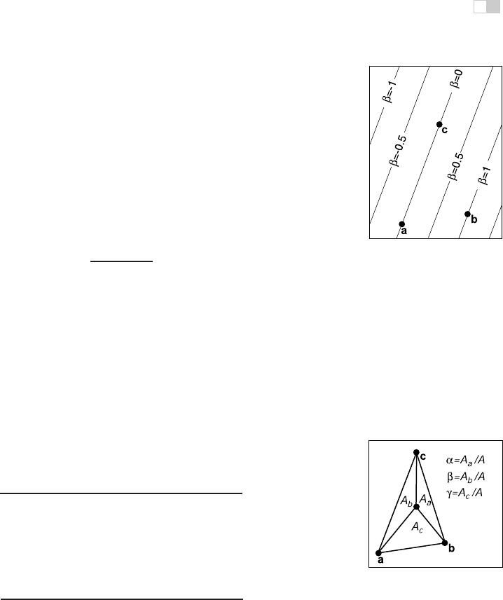
zero. There are analogous formulas for α and β, but typically only one is needed:
Figure 2.38. The bary-
centric coordinates are pro-
portional to the areas of the
three subtriangles shown.
β =
(y
a
− y
c
)x +(x
c
− x
a
)y + x
a
y
c
− x
c
y
a
(y
a
− y
c
)x
b
+(x
c
− x
a
)y
b
+ x
a
y
c
− x
c
y
a
,
α =1− β − γ.
Another way to compute barycentric coordinates is to compute the areas A
a
, A
b
,
and A
c
, of subtriangles as shown in Figure 2.38. Barycentric coordinates obey
the rule
α = A
a
/A,
β = A
b
/A,
γ = A
c
/A,
(2.34)
..................Content has been hidden....................
You can't read the all page of ebook, please click here login for view all page.