

i
i
i
i
i
i
i
i
400 16. Implicit Modeling
+
+
+
-
-
-
-
-
+
+
+
-
-
-
-
-
+
-
-
+
-
-
Figure 16.14. Examples of vertices inside (+) and outside (-) the surface. Note the extra
sample gives a clue to avoid ambiguous cases.
16.3.4 Sampling Problems
Ambiguities occur when opposite corners of a face (or the cube) have the same
sign and the other pair of vertices on the face have the opposite sign (see Figure
16.14). A sample taken in the center of the face will give a clue as to whether the
-
-
+
+
Figure 16.15. Cube too
large to capture small vari-
ation in implicit function.
cube represents the meeting of two surfaces or a saddle. It should be made clear
that a spatial grid stores a sample of the implicit function at every vertex. If the
function happens to vary considerably within a cell the polygonal representation
will not show such variations (see Figure 16.15). The surface cannot be resolved
by sampling alone unless something is known about the curvature of the surface.
A good discussion of this topic appears in (Kalra & Barr, 1989).
This ambiguity problem (not the under-sampling problem) is avoided by sub-
dividing the cubic cell into tetrahedra. The tetrahedra can then be polygonized
unambiguously. Since there are four vertices in each tetrahedron, a table of six-
teen entries will provide the correct triangle information. The disadvantage is that
approximately twice the number of polygons will be generated.
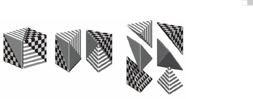
Subdividing a Cube
Without requiring additional cell vertices, a cube may be decomposed into five or
six tetrahedra as shown in Figure 16.16. These decompositions introduce diago-
nals on the cube faces, and to maintain a consistent diagonal direction between
i
i
i
i
i
i
i
i
16.4. More on Blending 401
Figure 16.16. Decomposing a cube into six tetrahedra.
Image courtesy Erwin DeGroot
.
neighbors, the six decomposition is preferable. The introduction of diagonal
edges produces a higher-resolution surface than replacing each cube directly with
triangles. The decomposition into tetrahedra and the replacement of the tetrahe-
dra with triangles are fast, table-driven algorithms, which produce topologically
consistent meshes.
16.3.5 Cell Polygonization
Two obvious problems emerge from the use of uniform space subdivision. The
size of triangles output by this algorithm do not adapt to the curvature of the sur-
face and a further sample is required to solve the ambiguities, in which cubic cells
are replaced by polygons. A space subdivision algorithm based on an octree was
developed by Bloomenthal (Bloomenthal, 1988), which does adapt to the curva-
ture of the surface. Cells are subdivided into eight octants and cracks are avoided
by using a restricted octree scheme, i.e., neighboring cells cannot differ by more
than one level of subdivision. This indeed reduces the number of polygons gen-
erated, but full advantage of large cells can only be taken if the flat regions of
the surface happen to fall entirely within the appropriate octants. The algorithm
proves in practice to be considerably slower than the uniform voxel algorithm and
is more complicated to implement.
16.4 More on Blending
Section 16.1 showed that blending can be made to occur when field values are
summed. Ricci, in his landmark paper (Ricci, 1973), describes super-elliptic

i
i
i
i
i
i
i
i
402 16. Implicit Modeling
blending. Given two functions F
A
and F
B
, previously we simply found the im-
plicit value as F
total
= F
A
+ F
B
. We can denote this more general blending
operator as A B. The Ricci blend is defined as:
f
AB
=(f
A
n
+ f
B
n
)
1
n
. (16.4)
It is interesting to point out the following properties:
lim
n→+∞
(f
A
n
+ f
B
n
)
1
n
=max(f
A
,f
B
),
lim
n→−∞
(f
A
n
+ f
B
n
)
1
n
=min(f
A
,f
B
).
Figure 16.17. By varying
n
, the Ricci blend may be
made to change smoothly
from blend to union.
Image
courtesy Erwin DeGroot
.
Moreover,this generalized blendingis associative, i.e., f
(AB)C
= f
A(BC)
.
The standard blending operator + proves to be a special case of the super-elliptic
blend with n =1.Whenn varies from 1 to infinity, it creates a set of blends
interpolating between blending A + B and union A ∪B (see Figure 16.17). Fig-
ure 16.27 shows the nodes to be binary or unary; in fact the binary nodes can
easily be extended using the above formulation to n-ary nodes.
The power of Ricci’s operators is that they are closed under the operations
on the space of all possible implicit volumes, meaning that an application of an
operator simply produces another scalar field defining another implicit volume.
This new field can be composed with other fields, again using Ricci’s operators.
Equation (16.4) will always produce the exact union of two implicit volumes,
regardless of how complex they are. Compared with the difficulties involved in
applying boolean CSG operations to B-rep surfaces, solid modeling with implicit
volumes is incredibly simple.
Following Pasko’s functional representation (A. Pasko et al., 1995), another
generalized blending function may be defined:
f
AB
=
f
A
+ f
B
+ α
f
A
2
+ f
B
2
f
A
2
+ f
B
2
n
2
.
When α ∈ [−1, 1] varies from −1 to 1, it creates a set of blends interpolating
the union and the intersection operators. However, this operator is no longer
associative which is incompatible with the definition of n-ary operators.
16.5 Constructive Solid Geometry
Implicit models are frequently termed implicit surfaces; however, they are inher-
ently volume models and useful for solid modeling operations. Ricci introduced a
constructive geometry for defining complex shapes from operationssuch as union,
i
i
i
i
i
i
i
i
16.5. Constructive Solid Geometry 403
intersection, difference, and blend upon primitives (Ricci, 1973). The surface was
considered as the boundary between the half spaces f(p) < 1,defining the in-
side, and f(p) > 1 defining the outside. This initial approach to solid modeling
evolved into constructive solid geometry or CSG (Ricci, 1973; Requicha, 1980).
CSG is typically evaluated bottom-up according to a binary tree, with low-degree
polynomial primitives as the leaf nodes and internal nodes representing Boolean
set operations. These methods are readily adapted for use in implicit modeling,
and in the case of skeletal implicit surfaces, the Boolean set operations union
∪
max
, intersection ∩
min
and difference
minmax
are defined as follows (Wyvill et
al., 1999):
∪
max
f =
k−1
max
i=0
(f
i
) , (16.5)
∩
min
f =
k−1
min
i=0
(f
i
) ,
minmax
f =min
f
0
, 2 ∗iso −
k−1
max
j=1
(f
j
)
.
The Ricci operators are illustrated in Figure 16.18 for point primitives A
and B. For union (bottom left) the field at all points inside the union will be the
greater of f
A
() and f
B
(). For intersection (center), points in the region marked
as P
1
will have value min (f
A
(P
1
),f
B
(P
1
)) = 0, since the contribution of B will
be zero outside of its range of influence. Similarly, for the region marked as P
2
,
(influence of A is zero, i.e., the minimum) leaving only the intersection region
with positive values. Difference works similarly using the iso-value in the three
marked regions (P
i
) as follows:
f(P
0
)=min(f
B
(P
0
), 2 ∗ iso − f
A
(P
0
))
= min([iso, 1], [2 ∗ iso −1, iso])
=[2∗iso −1, iso] < iso
f(P
1
)=min(f
B
(P
1
), 2 ∗ iso − f
A
(P
1
))
=min([0, iso], [2 ∗ iso − 1, iso]) < iso
f(P
2
)=min(f
B
(P
2
), 2 ∗ iso − f
A
(P
2
))
= min([iso, 1], [iso, 2 ∗ iso]) >=iso
CSG operators create creases, i.e., C
1
discontinuities. For example, the min()
operator (Equation (16.5)) creates C
1
discontinuities at all points where f
1
(p)=
f
2
(p). When applied to two spheres, the discontinuities produced by this union
operator result in a crease on the surface, as shown in Figure 16.18, which is
the desired result. Discontinuities unfortunately extend into the field outside of

i
i
i
i
i
i
i
i
404 16. Implicit Modeling
P
1
P
0
P
2
Figure 16.18. Ricci operators for CSG.
Image courtesy Erwin DeGroot
.
the surface, which is not visible in this image. If a blend is then applied to the
result of the union, the C
1
-discontinuous plane in the field produces a shading
discontinuity (Figure 16.19).
Crease
Figure 16.19. Two
point primitives on the left
are connected by the Ricci
union. A third primitive is
blended to the result, creat-
ing an unwanted crease in
the field.
Image courtesy
Erwin DeGroot
.
The problem can be avoided to an extent (G. Pasko et al., 2002), and CSG op-
erators have been developed that are C
1
at all points except those where f
1
(p)=
f
2
(p)=iso(Barthe et al., 2003).
16.6 Warping
The ability to distort the shape of a surface by warping the space in its neigh-
borhood is a useful modeling tool. A warp is a continuous function w(x, y, z)
that maps R
3
onto R
3
. Sederberg provides a good analogy for warping when de-
scribing free form deformations (Sederberg & Parry, 1986). He suggests that the
warped space can be likened to a clear, flexible, plastic parallelepiped in which
the objects to be warped are embedded. A warped element may be defined by
simply applying some warp function w(p) to the implicit equation:
f
i
(x, y, z)=g
i
◦ d
i
◦ w
i
(x, y, z). (16.6)
A warped element may be fully characterized by the distance to its skele-
ton d
i
(x, y, z), its fall-off filter function g
i
(r), and eventually its warp function
w
i
(x, y, z). To render or perform operations on an implicit surface, the implicit
P
Q
Figure 16.20. Point
Q
returns the field value for
point
P
.
value of many points f(P ) must be found. First, P is transformed by the warp
function to some new point Q,andf(Q) is returned in place of f (P ).InFig-
ure 16.20, instead of returning the implicit value of some point f (Q),thevalue
..................Content has been hidden....................
You can't read the all page of ebook, please click here login for view all page.