

i
i
i
i
i
i
i
i
248 11. Texture Mapping
by using a sort of “solid noise,” usually called Perlin noise after its inventor, who
received a technical Academy Award for its impact in the film industry (Perlin,
1985).
Getting a noisy appearance by calling a random number for every point would
not be appropriate, because it would just be like “white noise” in TV static. We
would like to make it smoother without losing the random quality. One possibility
is to blur white noise, but there is no practical implementation of this. Another
possibility is to make a large lattice with a random number at every lattice point,
and then interpolate these random points for new points between lattice nodes;
this is just a 3D texture array as described in the last section with random numbers
in the array. This technique makes the lattice too obvious. Perlin used a variety
of tricks to improve this basic lattice technique so the lattice was not so obvious.
This results in a rather baroque-looking set of steps, but essentially there are just
three changes from linearly interpolating a 3D array of random values. The first
change is to use Hermite interpolation to avoid mach bands, just as can be done
with regular textures. The second change is the use of random vectors rather than
values, with a dot product to derive a random number; this makes the underlying
grid structure less visually obvious by moving the local minima and maxima off
the grid vertices. The third change is to use a 1D array and hashing to create a
virtual 3D array of random vectors. This adds computation to lower memory use.
Here is his basic method:
n(x, y, z)=
x+1
i=x
y+1
j=y
z+1
k=z
Ω
ijk
(x − i, y −j, z − k),
where (x, y, z) are the Cartesian coordinates of x,and
Ω
ijk
(u, v, w)=ω(u)ω(v)ω(w)(Γ
ijk
· (u, v, w)) ,
and ω(t) is the cubic weighting function:
ω(t)=
2|t|
3
− 3|t|
2
+1 if |t| < 1,
0 otherwise.
Figure 11.4. Absolute
value of solid noise, and
noise for scaled
x
and
y
val-
ues.
The final piece is that Γ
ijk
is a random unit vector for the lattice point(x, y, z)=
(i, j, k). Since we want any potential ijk, we use a pseudorandom table:
Γ
ijk
= G (φ(i + φ(j + φ(k)))) ,
where G is a precomputed array of n random unit vectors, and φ(i)=
P [i mod n] where P is an array of length n containing a permutation of the

i
i
i
i
i
i
i
i
11.1. 3D Texture Mapping 249
integers 0 through n − 1. In practice, Perlin reports n = 256 works well. To
choose a random unit vector (v
x
,v
y
,v
z
) first set
v
x
=2ξ − 1,
v
y
=2ξ
− 1,
v
z
=2ξ
− 1,
where ξ, ξ
,ξ
are canonical random numbers (uniform in the interval [0, 1)).
Then, if (v
2
x
+v
2
y
+v
2
z
) < 1, make the vector a unit vector. Otherwise keep setting
it randomly until its length is less than one, and then make it a unit vector. This
is an example of a rejection metho d, which will be discussed more in Chapter 14.
Essentially, the “less than” test gets a random point in the unit sphere, and the
vector for the origin to that point is uniformly random. That would not be true of
random points in the cube, so we “get rid” of the corners with the test.
Because solid noise can be positive or negative, it must be transformed before
being converted to a color. The absolute value of noise over a ten by ten square is
shown in Figure 11.4, along with stretched versions. There versions are stretched
by scaling the points input to the noise function.
Figure 11.5. Using
0.5(noise+1) (top) and
0.8(noise+1) (bottom) for
intensity.
The dark curves are where the original noise function changed from positive
to negative. Since noise varies from −1 to 1, a smoother image can be achieved
by using (noise+1)/2 for color. However, since noise values close to 1 or −1 are
rare, this will be a fairly smooth image. Larger scaling can increase the contrast
(Figure 11.5).
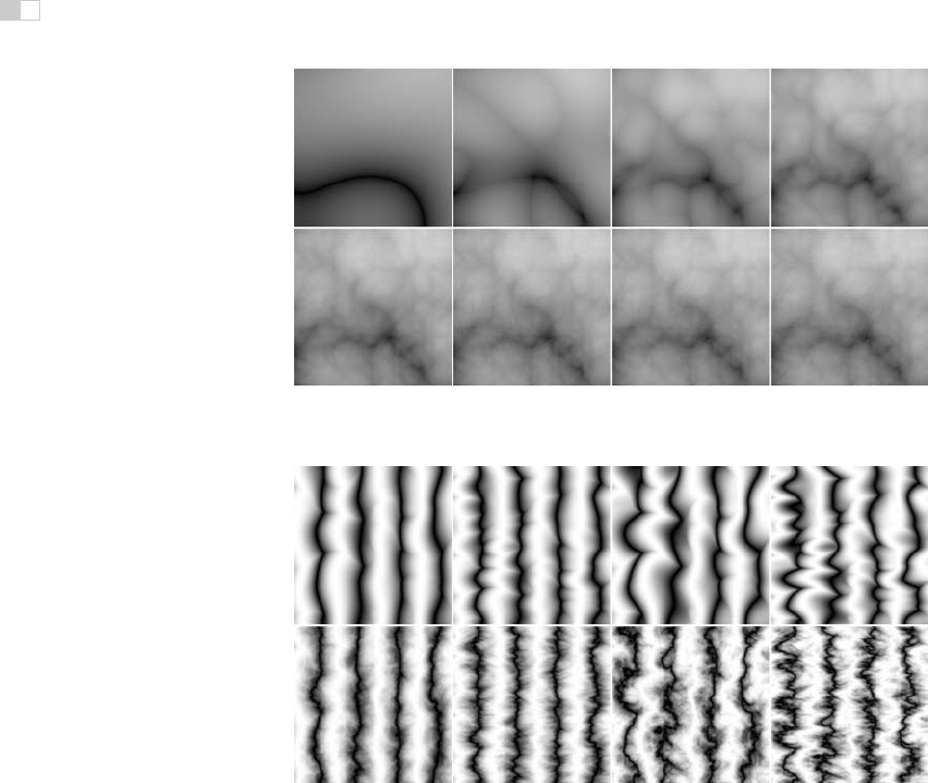
11.1.4 Turbulence
Many natural textures contain a variety of feature sizes in the same texture. Perlin
uses a pseudofractal “turbulence” function:
n
t
(x)=
i
|n(2
i
x)|
2
i
This effectively repeatedly adds scaled copies of the noise function on top of itself
as shown in Figure 11.6.
The turbulence can be used to distort the stripe function:
RGB turbstripe( point p, double w )
double t =(1+sin(k
1
z
p
+ turbulence(k
2
p))/w)/2
return t ∗ s0+(1− t) ∗ s1
Various values for k
1
and k
2
were used to generate Figure 11.7.
i
i
i
i
i
i
i
i
250 11. Texture Mapping
Figure 11.6. Turbulence function with (from top left to bottom right) one through eight terms
in the summation.
Figure 11.7. Various turbulent stripe textures with different
k
1
,
k
2
. The top row has only the
first term of the turbulence series.
11.2 2D Texture Mapping
For 2D texture mapping, we use a 2D coordinate, often called uv, which is used
to create a reflectance R(u, v). The key is to take an image and associate a (u, v)
coordinate system on it so that it can, in turn, be associated with points on a 3D
surface. For example, if the latitudes and longitudes on the world map are associ-
ated with a polar coordinate system on the sphere, we get a globe (Figure 11.8).
It is crucial that the coordinates on the image and the object match in “just the
right way.” As a convention, the coordinate system on the image is set to be the
unit square (u, v) ∈ [0, 1]
2
.For(u, v) outside of this square, only the fractional
parts of the coordinates are used resulting in a tiling of the plane (Figure 11.2).

i
i
i
i
i
i
i
i
11.2. 2D Texture Mapping 251
Figure 11.8. A Miller cylindrical projection map world map and its placement on the sphere.
The distortions in the texture map (i.e., Greenland being so large) exactly correspond to the
shrinking that occurs when the map is applied to the sphere.
Note that the image has a different number of pixels horizontally and vertically,
so the image pixels have a non-uniform aspect ratio in (u, v) space.
To map this (u, v) ∈ [0, 1]
2
image onto a sphere, we first compute the polar
coordinates. Recall the spherical coordinate system described by Equation (2.25).
For a sphere of radius R with center (c
x
,c
y
,c
z
), the parametric equation of the
sphere is
x = x
c
+ R cos φ sin θ,
y = y
c
+ R sin φ sin θ,
z = z
c
+ R cos θ.
We can find (θ, φ):
θ = arccos
z − z
c
R
,
φ = arctan2(y − y
c
,x− x
c
),
where arctan2(a, b) is the the atan2 of most math libraries which returns the
arctangent of a/b. Because (θ, φ) ∈ [0,π] × [−π, π],weconvertto(u, v) as
follows, after first adding 2π to φ if it is negative:
u =
φ
2π
,
v =
π − θ
π
.
This mapping is shown in Figure 11.8. There is a similar, although likely more
complicated way, to generate coordinates for most 3D shapes.

i
i
i
i
i
i
i
i
252 11. Texture Mapping
11.3 Texture Mapping for Rasterized Triangles
For surfaces represented by triangle meshes, texture coordinates are defined by
storing (u, v) texture coordinates at each vertex of the mesh (see Section 12.1).
So, if a triangle is intersected at barycentric coordinates (β,γ), you interpolate
the (u, v) coordinates the same way you interpolate points. Recall that the point
at barycentric coordinate (β,γ) is
p(β,γ)=a + β(b − a)+γ(c −a).
A similar equation applies for (u, v):
u(β,γ)=u
a
+ β(u
b
− u
a
)+γ(u
c
− u
a
),
v(β,γ)=v
a
+ β(v
b
− v
a
)+γ(v
c
− v
a
).
Several ways a texture can be applied by changing the (u, v) at triangle ver-
tices are shown in Figure 11.10. This sort of calibration texture map makes it
easier to understand the texture coordinates of your objects during debugging
(Figure 11.9).
Figure 11.9. Top: a cal-
ibration texture map. Bot-
tom: the sphere viewed
along the
y
-axis.
We would like to get the same texture images whether we use a ray tracing
program or a rasterization method, such as a z-buffer. There are some subtleties in
achieving this with correct-looking perspective, but we can address this at the ras-
terization stage. The reason things are not straightforward is that just interpolating
Figure 11.10. Various mesh textures obtained by changing (
u,v
) coordinates stored at
vertices.
..................Content has been hidden....................
You can't read the all page of ebook, please click here login for view all page.