
i
i
i
i
i
i
i
i
12.4. BSP Trees for Visibility 291
and for all points p
−
on the other side of the plane, f
1
(p
−
) < 0. Using this
property, we can find out on which side of the plane T
2
lies. Again, this assumes
all three vertices of T
2
are on the same side of the plane. For discussion, assume
that T
2
is on the f
1
(p) < 0 side of the plane. Then, we can draw T
1
and T
2
in the
right order for any eyepoint e:
if (f
1
(e) < 0) then
draw T
1
draw T
2
else
draw T
2
draw T
1
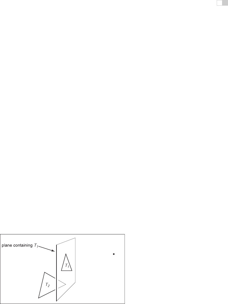
The reason this works is that if T
2
and e are on the same side of the plane con-
taining T
1
, there is no way for T
2
to be fully or partially blocked by T
1
as seen
from e,soitissafetodrawT
1
first. If e and T
2
are on opposite sides of the
plane containing T
1
,thenT
2
cannot fully or partially block T
1
, and the opposite
drawing order is safe (Figure 12.35).
This observation can be generalized to many objects provided none of them
span the plane defined by T
1
. If we use a binary tree data structure with T
1
as root, the negative branch of the tree contains all the triangles whose
vertices have f
i
(p) < 0,andthepositive branch of the tree contains all the
triangles whose vertices have f
i
(p) > 0. We can draw in proper order
as follows:
function draw(bsptree tree, point e)
if (tree.empty) then
return
e
Figure 12.35. When e and
T
2
are on opposite sides of the plane containing
T
1
, then it is
safe to draw
T
2
first and
T
1
second. If e and
T
2
are on the same side of the plane, then
T
1
should be drawn before
T
2
. This is the core idea of the BSP tree algorithm.

i
i
i
i
i
i
i
i
292 12. Data Structures for Graphics
if (f
tree.root
(e) < 0) then
draw(tree.plus, e)
rasterize tree.triangle
draw(tree.minus, e)
else
draw(tree.minus, e)
rasterize tree.triangle
draw(tree.plus, e)
The nice thing about that code is that it will work for any viewpoint e,sothe
tree can be precomputed. Note that, if each subtree is itself a tree, where the root
triangle divides the other triangles into two groups relative to the plane containing
it, the code will work as is. It can be made slightly more efficient by terminat-
ing the recursive calls one level higher, but the code will still be simple. A tree
illustrating this code is shown in Figure 12.36. As discussed in Section 2.5.5, the
implicit equation for a point p on a plane containing three non-colinear points a,
b,andc is
f(p)=((b − a) × (c − a)) · (p − a)=0. (12.1)
Figure 12.36. Three triangles and a BSP tree that is valid for them. The “positive” and
“negative” are encoded by right and left subtree position, respectively.
i
i
i
i
i
i
i
i
12.4. BSP Trees for Visibility 293
It can be faster to store the (A, B, C, D) of the implicit equation of the form
f(x, y, z)=Ax + By + Cz + D =0. (12.2)
Equations (12.1) and (12.2) are equivalent, as is clear when you recall that the
gradient of the implicit equation is the normal to the triangle. The gradient of
Equation (12.2) is n =(A, B, C) which is just the normal vector
n =(b − a) × (c − a).
We can solve for D by plugging in any point on the plane, e.g., a:
D = −Ax
a
− By
a
− Cz
a
= −n · a.
This suggests the form:
f(p)=n · p − n · a
= n ·(p −a)
=0,
which is the same as Equation (12.1) once you recall that n is computed using the
cross product. Which form of the plane equation you use and whether you store
only the vertices, n and the vertices, or n, D, and the vertices, is probably a matter
of taste—a classic time-storage tradeoff that will be settled best by profiling. For
debugging, using Equation (12.1) is probably the best.
The only issue that prevents the code above from working in general is that
one cannot guarantee that a triangle can be uniquely classified on one side of a
plane or the other. It can have two vertices on one side of the plane and the third
on the other. Or it can have vertices on the plane. This is handled by splitting the
triangle into smaller triangles using the plane to “cut” them.
12.4.2 Building the Tree
If none of the triangles in the dataset cross each other’s planes, so that all triangles
are on one side of all other triangles, a BSP tree that can be traversed using the
code above can be built using the following algorithm:
tree-root = node(T
1
)
for i ∈{2,...,N} do
tree-root.add(T
i
)

i
i
i
i
i
i
i
i
294 12. Data Structures for Graphics
function add ( triangle T )
if (f(a) < 0 and f(b) < 0 and f(c) < 0) then
if (negative subtree is empty) then
negative-subtree = node(T )
else
negative-subtree.add (T )
else if (f(a) > 0 and f(b) > 0 and f(c) > 0) then
if positive subtree is empty then
positive-subtree = node(T )
else
positive-subtree.add (T )
else
we have assumed this case is impossible
a
b
c
A
B
Figure 12.37. Whenatri-
angle spans a plane, there
will be one vertex on one
side and two on the other.
The only thing we need to fix is the case where the triangle crosses the dividing
plane, as shown in Figure 12.37. Assume, for simplicity, that the triangle has
vertices a and b on one side of the plane, and vertex c is on the other side. In this
case, we can find the intersection points A and B and cut the triangle into three
new triangles with vertices
T
1
=(a, b, A),
T
2
=(b, B , A),
T
3
=(A, B, c),
as shown in Figure 12.38. This order of vertices is important so that the direction
of the normal remains the same as for the original triangle. If we assume that
f(c) < 0, the following code could add these three triangles to the tree assuming
the positive and negative subtrees are not empty:
positive-subtree = node (T
1
)
positive-subtree = node (T
2
)
negative-subtree = node (T
3
)
A precision problem that will plague a naive implementation occurs when a vertex
is very near the splitting plane. For example, if we have two vertices on one side of
the splitting plane and the other vertex is only an extremely small distance on the
Figure 12.38. When a
triangle is cut, we break it
into three triangles, none
of which span the cutting
plane.
other side, we will create a new triangle almost the same as the old one, a triangle
that is a sliver, and a triangle of almost zero size. It would be better to detect this
as a special case and not split into three new triangles. One might expect this case
to be rare, but because many models have tessellated planes and triangles with
i
i
i
i
i
i
i
i
12.4. BSP Trees for Visibility 295
shared vertices, it occurs frequently, and thus must be handled carefully. Some
simple manipulations that accomplish this are:
function add( triangle T )
fa = f (a)
fb = f(b)
fc = f(c)
if (abs(fa) <) then
fa = 0
if (abs(fb) <) then
fb = 0
if (abs(fc) <) then
fc = 0
if (fa ≤ 0 and fb ≤ 0 and fc ≤ 0) then
if (negative subtree is empty) then
negative-subtree = node(T )
else
negative-subtree.add(T )
else if (fa ≥ 0 and fb ≥ 0 and fc ≥ 0) then
if (positive subtree is empty) then
positive-subtree = node(T )
else
positive-subtree.add(T )
els
e
cut triangle into three triangles and add to each side
This takes any vertex whose f value is within of the plane and counts it as
positive or negative. The constant is a small positive real chosen by the user.
The technique above is a rare instance where testing for floating-point equality is
useful and works because the zero value is set rather than being computed. Com-
paring for equality with a computed floating-point value is almost never advisable,
but we are not doing that.
12.4.3 Cutting Triangles
Filling out the details of the last case “cut triangle into three triangles and add to
each side” is straightforward, but tedious. We should take advantage of the BSP
tree construction as a preprocess where highest efficiency is not key. Instead, we
should attempt to have a clean compact code. A nice trick is to force many of the
cases into one by ensuring that c is on one side of the plane and the other two
vertices are on the other. This is easily done with swaps. Filling out the details
..................Content has been hidden....................
You can't read the all page of ebook, please click here login for view all page.