

i
i
i
i
i
i
i
i
276 12. Data Structures for Graphics
In addition to the simple traversal algorithms shown in this chapter, all three of
these mesh topology structures can support “mesh surgery” operations of various
sorts, such as splitting or collapsing vertices, swapping edges, adding or removing
triangles, etc.
12.2 Scene Graphs
A triangle mesh manages a collection of triangles that constitute an object in a
scene, but another universal problem in graphics applications is arranging the
objects in the desired positions. As we saw in Chapter 6, this is done using trans-
formations, but complex scenes can contain a great many transformations and
organizing them well makes the scene much easier to manipulate. Most scenes
admit to a hierarchical organization, and the transformations can be managed ac-
cording to this hierarchy using a scene graph.
To motivate the scene-graph data structure, we will use the hinged pendulum
shown in Figure 12.19. Consider how we would draw the top part of the pendu-
lum:
M
1
= rotate(θ)
M
2
= translate(p)
M
3
= M
2
M
1
Apply M
3
to all points in upper pendulum
The bottom is more complicated, but we can take advantage of the fact that it is
attached to the bottom of the upper pendulum at point b in the local coordinate
system. First, we rotate the lower pendulum so that it is at an angle φ relative to
Figure 12.19. A hinged pendulum. On the left are the two pieces in their “local” coordinate
systems. The hinge of the bottom piece is at point b and the attachment for the bottom piece
is at its local origin. The degrees of freedom for the assembled object are the angles (θ,φ)
and the location p of the top hinge.

i
i
i
i
i
i
i
i
12.2. Scene Graphs 277
its initial position. Then, we move it so that its top hinge is at point b. Now it is
Figure 12.20. The scene
graph for the hinged pendu-
lum of Figure 12.19.
at the appropriate position in the local coordinates of the upper pendulum, and it
can then be moved along with that coordinate system. The composite transform
for the lower pendulum is:
M
a
= rotate(φ)
M
b
= translate(b)
M
c
= M
b
M
a
M
d
= M
3
M
c
Apply M
d
to all points in lower pendulum
Thus, we see that the lower pendulum not only lives in its own local coordinate
system, but also that coordinate system itself is moved along with that of the upper
pendulum.
Figure 12.21. Aferry,
a car on the ferry, and
the wheels of the car (only
two shown) are stored in a
scene-graph.
We can encode the pendulum in a data structure that makes management of
these coordinate system issues easier, as shown in Figure 12.20. The appropriate
matrix to apply to an object is just the product of all the matrices in the chain from
the object to the root of the data structure. For example, consider the model of a
ferry that has a car that can move freely on the deck of the ferry, and wheels that
each move relative to the car as shown in Figure 12.21.
As with the pendulum, each object should be transformed by the product of
the matrices in the path from the root to the object:
• ferry transform using M
0
• car body transform using M
0
M
1
• left wheel transform using M
0
M
1
M
2
• left wheel transform using M
0
M
1
M
3
An efficient implementation can be achieved using a matrix stack, a data structure
supported by many APIs. A matrix stack is manipulated using push and pop op-
erations that add and delete matrices from the right-hand side of a matrix product.
For example, calling:
push(M
0
)
push(M
1
)
push(M
2
)
creates the active matrix M = M
0
M
1
M
2
. A subsequent call to pop() strips the
last matrix added so that the active matrix becomes M = M
0
M
1
. Combining
the matrix stack with a recursive traversal of a scene graph gives us:

i
i
i
i
i
i
i
i
278 12. Data Structures for Graphics
function traverse(node)
push(M
local
)
draw object using composite matrix from stack
traverse(left child)
traverse(right child)
pop()
There are many variations on scene graphs but all follow the basic idea above.
12.3 Spatial Data Structures
In many, if not all, graphics applications, the ability to quickly locate geometric
objects in particular regions of space is important. Ray tracers need to find objects
that intersect rays; interactive applications navigating an environment need to find
the objects visible from any given viewpoint; games and physical simulations re-
quire detecting when and where objects collide. All these needs can be supported
by various spatial data structures designed to organize objects in space so they
can be looked up efficiently.
In this section we will discuss examples of three general classes of spatial data
structures. Structures that group objects together into a hierarchy are object par-
titioning schemes: objects are divided into disjoint groups, but the groups may
end up overlapping in space. Structures that divide space into disjoint regions
are space partitioning schemes: space is divided into separate partitions, but one
object may have to intersect more than one partition. Space partitioning schemes
can be regular, in which space is divided into uniformly shaped pieces, or irregu-
lar, in which space is divided adaptively into irregular pieces, with smaller pieces
where there are more and smaller objects.
Figure 12.22. Left: a uniform partitioning of space. Right: adaptive bounding-box hierarchy.
Image courtesy David DeMarle.

i
i
i
i
i
i
i
i
12.3. Spatial Data Structures 279
We will use ray tracing as the primary motivation while discussing these struc-
tures, though they can all also be used for view culling or collision detection. In
Chapter 4, all objects were looped over while checking for intersections. For N
objects, this is an O(N) linear search and is thus slow for large scenes. Like most
search problems, the ray-object intersection can be computed in sub-linear time
using “divide and conquer” techniques, provided we can create an ordered data
structure as a preprocess. There are many techniques to do this.
This section discusses three of these techniques in detail: bounding volume hi-
erarchies (Rubin & Whitted, 1980; Whitted, 1980; Goldsmith & Salmon, 1987),
uniform spatial subdivision (Cleary et al., 1983; Fujimoto et al., 1986; Ama-
natides & Woo, 1987), and binary space partitioning (Glassner, 1984; Jansen,
1986; Havran, 2000). An example of the first two strategies is shown in Fig-
ure 12.22.
12.3.1 Bounding Boxes
A key operation in most intersection-acceleration schemes is computing the in-
tersection of a ray with a bounding box (Figure 12.23). This differs from conven-
tional intersection tests in that we do not need to know where the ray hits the box;
we only need to know whether it hits the box.
To build an algorithm for ray-box intersection, we begin by considering a 2D
ray whose direction vector has positive x and y components. We can generalize
this to arbitrary 3D rays later. The 2D bounding box is defined by two horizontal
and two vertical lines:
Figure 12.23. The ray is
only tested for intersection
with the surfaces if it hits the
bounding box.
x = x
min
,
x = x
max
,
y = y
min
,
y = y
max
.
The points bounded by these lines can be described in interval notation:
(x, y) ∈ [x
min
,x
max
] × [y
min
,y
max
].
As shown in Figure 12.24, the intersection test can be phrased in terms of these
intervals. First, we compute the ray parameter where the ray hits the line x =
x
min
:
t
xmin
=
x
min
− x
e
x
d
.
i
i
i
i
i
i
i
i
280 12. Data Structures for Graphics
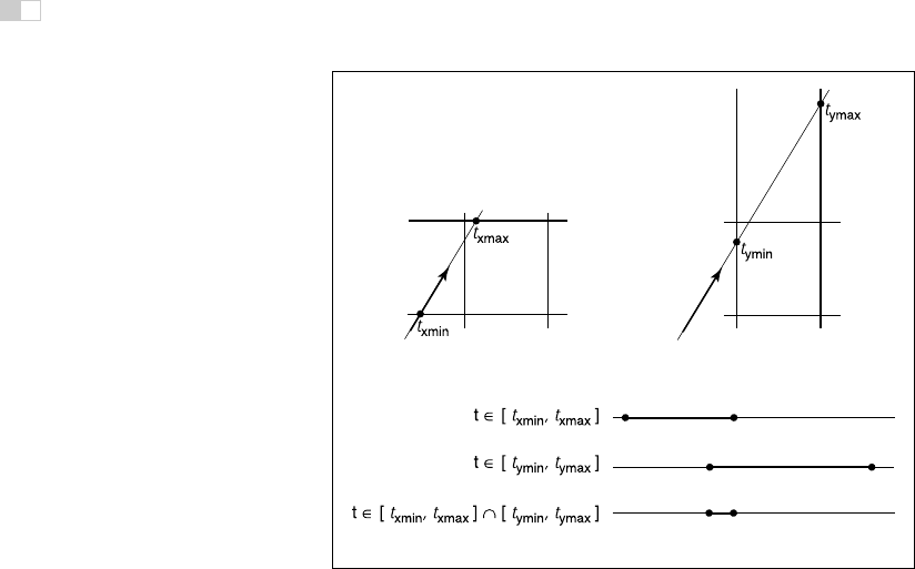
Figure 12.24. The ray will be inside the interval
x
∈ [
x
min
,
x
max
] for some interval in its
parameter space
t
∈ [
t
xmin
,
t
xmax
]. A similar interval exists for the
y
interval. The ray intersects
the box if it is in both the
x
interval and
y
interval at the same time, i.e., the intersection of the
two one-dimensional intervals is not empty.
We then make similar computations for t
xmax
, t
ymin
,andt
ymax
. The ray hits the
box if and only if the intervals [t
xmin
,t
xmax
] and [t
ymin
,t
ymax
] overlap, i.e., their
intersection is non-empty. In pseudocode this algorithm is:
t
xmin
=(x
min
− x
e
)/x
d
t
xmax
=(x
max
− x
e
)/x
d
t
ymin
=(y
min
− y
e
)/y
d
t
ymax
=(y
max
− y
e
)/y
d
if (t
xmin
>t
ymax
) or (t
ymin
>t
xmax
) then
return false
else
return true
The if statement may seem non-obvious. To see the logic of it, note that there is
no overlap if the first interval is either entirely to the right or entirely to the left of
the second interval.
The first thing we must address is the case when x
d
or y
d
is negative. If x
d
is
negative, then the ray will hit x
max
before it hits x
min
. Thus the code for computing
..................Content has been hidden....................
You can't read the all page of ebook, please click here login for view all page.