

i
i
i
i
i
i
i
i
13.4. Distribution Ray Tracing 313
This shuffle routine eliminates any coherence between arrays r and s.Theshadow
routine will just use the 2D random point stored in s[p] rather than calling the
random number generator. A shuffle routine for an array indexed from 0 to N −1
is:
for i = N −1 downto 1 do
choose random integer j between 0 and i inclusive
swap array elements i and j
13.4.3 Depth of Field
The soft focus effects seen in most photos can be simulated by collecting light at
a non-zero size “lens” rather than at a point. This is called depth of field.The
lens collects light from a cone of directions that has its apex at a distance where
everythingis in focus (Figure 13.15). We can place the “window” we are sampling
on the plane where everything is in focus (rather than at the z = n plane as we did
previously) and the lens at the eye. The distance to the plane where everything is
in focus we call the focus plane, and the distance to it is set by the user, just as the
distance to the focus plane in a real camera is set by the user or range finder.
Figure 13.15. The lens
averages over a cone of
directions that hit the pixel
location being sampled.
Figure 13.16. An example of depth of field. The caustic in the shadow of the wine glass is
computed using particle tracing as described in Chapter 24. (See also Plate V.)
i
i
i
i
i
i
i
i
314 13. More Ray Tracing
To be most faithful to a real camera, we should make the lens a disk. However,
we will get very similar effects with a square lens (Figure 13.17). So we choose
the side-length of the lens and take random samples on it. The origin of the
view rays will be these perturbed positions rather than the eye position. Again, a
shuffling routine is used to prevent correlation with the pixel sample positions. An
example using 25 samples per pixel and a large disk lens is shown in Figure 13.16.
Figure 13.17. To create
depth-of-field effects, the
eye is randomly selected
from a square region.
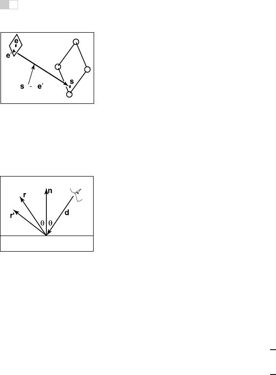
13.4.4 Glossy Reflection
Some surfaces, such as brushed metal, are somewhere between an ideal mirror
and a diffuse surface. Some discernible image is visible in the reflection but it
is blurred. We can simulate this by randomly perturbing ideal specular reflection
rays as shown in Figure 13.18.
Only two details need to be worked out: how to choose the vector r
and what
to do when the resulting perturbed ray is below the surface from which the ray is
reflected. The latter detail is usually settled by returning a zero color when the
ray is below the surface.
Figure 13.18. The re-
flection ray is perturbed to
a random vector r
.
To choose r
, we again sample a random square. This square is perpendicular
to r and has width a which controls the degree of blur. We can set up the square’s
orientation by creating an orthonormal basis with w = r using the techniques in
Section 2.4.6. Then, we create a random point in the 2D square with side length
a centered at the origin. If we have 2D sample points (ξ, ξ
) ∈ [0, 1]
2
, then the
analogous point on the desired square is
u = −
a
2
+ ξa,
v = −
a
2
+ ξ
a.
Because the square over which we will perturb is parallel to both the u and v
vectors, the ray r
is just
r
= r + uu + vv.
Note that r
is not necessarily a unit vector and should be normalized if your code
requires that for ray directions.
13.4.5 Motion Blur
We can add a blurred appearance to objects as shown in Figure 13.19. This is
called motion blur and is the result of the image being formed over a non-zero

i
i
i
i
i
i
i
i
13.4. Distribution Ray Tracing 315
Figure 13.19. The bottom right sphere is in motion, and a blurred appearance results.
Image courtesy Chad Barb.
span of time. In a real camera, the aperture is open for some time interval during
which objects move. We can simulate the open aperture by setting a time variable
ranging from T
0
to T
1
. For each viewing ray we choose a random time,
T = T
0
+ ξ(T
1
− T
0
).
We may also need to create some objects to move with time. For example, we
might have a moving sphere whose center travels from c
0
to c
1
during the interval.
Given T , we could compute the actual center and do a ray–intersection with that
sphere. Because each ray is sent at a different time, each will encounter the sphere
at a different position, and the final appearance will be blurred. Note that the
bounding box for the moving sphere should bound its entire path so an efficiency
structure can be built for the whole time interval (Glassner, 1988).
i
i
i
i
i
i
i
i
316 13. More Ray Tracing
Notes
There are many, many other advanced methods that can be implemented in the
ray-tracing framework. Some resources for further information are Glassner’s An
Introduction to Ray Tracing and Principles of Digital Image Synthesis,Shirley’s
Realistic Ray Tracing, and Pharr and Humphreys’s Physically Based Rendering:
From Theory to Implementation.
Frequently Asked Questions
• What is the best ray-intersection efficiency structure?
The most popular structures are binary space partitioning trees (BSP trees), uni-
form subdivision grids, and bounding volume hierarchies. Most people who use
BSP trees make the splitting planes axis-aligned, and such trees are usually called
k-d trees. There is no clear-cut answer for which is best, but all are much, much
better than brute-force search in practice. If I were to implement only one, it
would be the bounding volume hierarchy because of its simplicity and robustness.
• Why do people use bounding boxes rather than spheres or ellipsoids?
Sometimes spheres or ellipsoids are better. However, many models have polyg-
onal elements that are tightly bounded by boxes, but they would be difficult to
tightly bind with an ellipsoid.
..................Content has been hidden....................
You can't read the all page of ebook, please click here login for view all page.