
i
i
i
i
i
i
i
i
6.3. Translation and Affine Transformations 131
but this scheme also makes it obvious how to compose two affine transformations:
simply multiply the matrices.
A problem with this new formalism arises when we need to transform vec-
tors that are not supposed to be positions—they represent directions, or offsets
between positions. Vectors that represent directions or offsets should not change
when we translate an object. Fortunately, we can arrange for this by setting the
third coordinate to zero:
⎡
⎣
10x
t
01y
t
00 1
⎤
⎦
⎡
⎣
x
y
0
⎤
⎦
=
⎡
⎣
x
y
0
⎤
⎦
.
If there is a scaling/rotation transformation in the upper-left 2 × 2 entries of the
matrix, it will apply to the vector, but the translation still multiplies with the zero
and is ignored. Furthermore, the zero is copied into the transformed vector, so
direction vectors remain direction vectors after they are transformed.
This is exactly the behavior we want for vectors, so they fit smoothly into the
system: the extra (third) coordinate will be either 1 or 0 depending on whether we
are encoding a position or a direction. We actually do need to store the homoge-
This gives an explanation
for the name “homoge-
neous:” translation, rota-
tion, and scaling of posi-
tions and directions all fit
into a single system.
neous coordinate so we can distinguish between locations and other vectors. For
example,
⎡
⎣
3
2
1
⎤
⎦
is a location and
⎡
⎣
3
2
0
⎤
⎦
is a displacement or direction.
Later, when we do perspective viewing, we will see that it is useful to allow the
homogeneous coordinate to take on values other than one or zero.
Homogeneous coordinates are used nearly universally to represent transfor-
mations in graphics systems. In particular, homogeneous coordinates underlie the
Homogeneous coordinates
are also ubiquitous in com-
puter vision.
design and operation of renderers implemented in graphics hardware. We will see
in Chapter 7 that homogeneous coordinates also make it easy to draw scenes in
perspective, another reason for their popularity.
Homogeneous coordinates can be considered just a clever way to handle the
bookkeeping for translation, but there is also a different, geometric interpretation.
The key observation is that when we do a 3D shear based on the z-coordinate we
get this transform:
⎡
⎣
10x
t
01y
t
00 1
⎤
⎦
⎡
⎣
x
y
z
⎤
⎦
=
⎡
⎣
x + x
t
z
y + y
t
z
z
⎤
⎦
.
Note that this almost has the form we want in x and y for a 2D translation, but
has a z hanging around that doesn’t have a meaning in 2D. Now comes the key
i
i
i
i
i
i
i
i
132 6. Transformation Matrices
decision: we will add a coordinate z =1to all 2D locations. This gives us
⎡
⎣
10x
t
01y
t
00 1
⎤
⎦
⎡
⎣
x
y
1
⎤
⎦
=
⎡
⎣
x + x
t
y + y
t
1
⎤
⎦
.
By associating a (z =1)-coordinate with all 2D points, we now can encode trans-
lations into matrix form. For example, to first translate in 2D by (t
x
,t
y
) and then
rotate by angle φ we would use the matrix
M =
⎡
⎣
cos φ −sin φ 0
sin φ cos φ 0
001
⎤
⎦
⎡
⎣
10x
t
01y
t
00 1
⎤
⎦
.
Note that the 2D rotation matrix is now 3 ×3 with zeros in the “translation slots.”
With this type of formalism, which uses shears along z =1to encode translations,
we can represent any number of 2D shears, 2D rotations, and 2D translations as
one composite 3D matrix. The bottom row of that matrix will always be (0, 0, 1),
so we don’t really have to store it. We just need to remember it is there when we
multiply two matrices together.
In 3D, the same technique works: we can add a fourth coordinate, a homoge-
neous coordinate, and then we have translations:
⎡
⎢
⎢
⎣
100x
t
010y
t
001z
t
000 1
⎤
⎥
⎥
⎦
⎡
⎢
⎢
⎣
x
y
z
1
⎤
⎥
⎥
⎦
=
⎡
⎢
⎢
⎣
x + x
t
y + y
t
z + z
t
1
⎤
⎥
⎥
⎦
.
Again, for a direction vector, the fourth coordinate is zero and the vector is thus
unaffected by translations.
Example (Windowing transformations). Often in graphics we need to create a trans-
form matrix that takes points in the rectangle [x
l
,x
h
] × [y
l
,y
h
] to the rectangle
[x
l
,x
h
] × [y
l
,y
h
]. This can be accomplished with a single scale and translate in
sequence. However, it is more intuitive to create the transform from a sequence
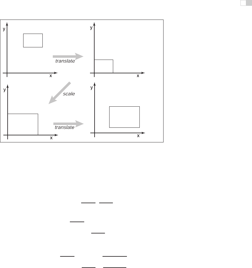
of three operations (Figure 6.18):
1. Move the point (x
l
,y
l
) to the origin.
2. Scale the rectangle to be the same size as the target rectangle.
3. Move the origin to point (x
l
,y
l
).
i
i
i
i
i
i
i
i
6.3. Translation and Affine Transformations 133
(x
l
, y
l
)
(x′
l
, y′
l
)
(x
h
, y
h
)
(x′
h
, y′
h
)
(x
h
– x
l
, y
h
– y
l
)
(x′
h
– x′
l
, y′
h
– y′
l
)
Figure 6.18. To take one rectangle (window) to the other, we first shift the lower-left corner
to the origin, then scale it to the new size, and then move the origin to the lower-left corner
of the target rectangle.
Remembering that the right-hand matrix is applied first, we can write
window = translate (x
l
,y
l
) scale
x
h
−x
l
x
h
−x
l
,
y
h
−y
l
y
h
−y
l
translate (−x
l
, −y
l
)
=
⎡
⎢
⎣
10x
l
01y
l
00 1
⎤
⎥
⎦
⎡
⎢
⎢
⎣
x
h
−x
l
x
h
−x
l
00
0
y
h
−y
l
y
h
−y
l
0
001
⎤
⎥
⎥
⎦
⎡
⎢
⎣
10−x
l
01−y
l
00 1
⎤
⎥
⎦
=
⎡
⎢
⎢
⎣
x
h
−x
l
x
h
−x
l
0
x
l
x
h
−x
h
x
l
x
h
−x
l
0
y
h
−y
l
y
h
−y
l
y
l
y
h
−y
h
y
l
y
h
−y
l
00 1
⎤
⎥
⎥
⎦
. (6.6)
It is perhaps not surprising to some readers that the resulting matrix has the form
it does, but the constructive process with the three matrices leaves no doubt as to
the correctness of the result.
An exactly analogous construction can be used to define a 3D windowing
transformation, which maps the box [x
l
,x
h
] × [y
l
,y
h
] × [z
l
,z
h
] to the box

i
i
i
i
i
i
i
i
134 6. Transformation Matrices
[x
l
,x
h
] × [y
l
,y
h
] × [z
l
,z
h
]:
⎡
⎢
⎢
⎢
⎢
⎢
⎣
x
h
−x
l
x
h
−x
l
00
x
l
x
h
−x
h
x
l
x
h
−x
l
0
y
h
−y
l
y
h
−y
l
0
y
l
y
h
−y
h
y
l
y
h
−y
l
00
z
h
−z
l
z
h
−z
l
z
l
z
h
−z
h
z
l
z
h
−z
l
000 1
⎤
⎥
⎥
⎥
⎥
⎥
⎦
. (6.7)
It is interesting to note that if we multiply an arbitrary matrix composed of
scales, shears, and rotations with a simple translation (translation comes second),
we get
⎡
⎢
⎢
⎣
100x
t
010y
t
001z
t
000 1
⎤
⎥
⎥
⎦
⎡
⎢
⎢
⎣
a
11
a
12
a
13
0
a
21
a
22
a
23
0
a
31
a
32
a
33
0
0001
⎤
⎥
⎥
⎦
=
⎡
⎢
⎢
⎣
a
11
a
12
a
13
x
t
a
21
a
22
a
23
y
t
a
31
a
32
a
33
z
t
0001
⎤
⎥
⎥
⎦
.
Thus, we can look at any matrix and think of it as a scaling/rotation part and a
translation part because the components are nicely separated from each other.
An important class of transforms are rigid-body transforms. These are com-
posed only of translations and rotations, so they have no stretching or shrinking
of the objects. Such transforms will have a pure rotation for the a
ij
above.
6.4 Inverses of Transformation Matrices
While we can always invert a matrix algebraically, we can use geometry if we
know what the transform does. For example, the inverse of scale(s
x
,s
y
,s
z
) is
scale(1/s
x
, 1/s
y
, 1/s
z
). The inverse of a rotation is the same rotation with the
opposite sign on the angle. The inverse of a translation is a translation in the
opposite direction. If we have a series of matrices M = M
1
M
2
···M
n
then
M
−1
= M
−1
n
···M
−1
2
M
−1
1
.
Also, certain types of transformation matrices are easy to invert. We’ve al-
ready mentioned scales, which are diagonal matrices; the second important ex-
ample is rotations, which are orthogonal matrices. Recall (Section 5.2.4) that the
inverse of an orthogonal matrix is its transpose. This makes it easy to invert ro-
tations and rigid body transformations (see Exercise 6). Also, it’s useful to know
that a matrix with [0 0 0 1] in the bottom row has an inverse that also has [0 0 0 1]
in the bottom row (see Exercise 7).
Interestingly, we can use SVD to invert a matrix as well. Since we know
that any matrix can be decomposed into a rotation times a scale times a rotation,

i
i
i
i
i
i
i
i
6.5. Coordinate Transformations 135
inversion is straightforward. For example in 3D we have
M = R
1
scale(σ
1
,σ
2
,σ
3
)R
2
,
and from the rules above it follows easily that
M
−1
= R
T
2
scale(1/σ
1
, 1/σ
2
, 1/σ
3
)R
T
1
.
6.5 Coordinate Transformations
All of the previous discussion has been in terms of using transformation matrices
to move points around. We can also think of them as simply changing the coor-
dinate system in which the point is represented. For example, in Figure 6.19, we
see two ways to visualize a movement. In different contexts, either interpretation
may be more suitable.
For example, a driving game may have a model of a city and a model of
a car. If the player is presented with a view out the windshield, objects inside
the car are always drawn in the same place on the screen, while the streets and
buildings appear to move backward as the player drives. On each frame, we
apply a transformation to these objects that moves them farther back than on the
previous frame. One way to think of this operation is simply that it moves the
buildings backward; another way to think of it is that the buildings are staying put
but the coordinate system in which we want to draw them—which is attached to
the car—is moving. In the second interpretation, the transformation is changing
Figure 6.19. The point (2,1) has a transform “translate by (-1,0)” applied to it. On the top
right is our mental image if we view this transformation as a physical movement, and on the
bottom right is our mental image if we view it as a change of coordinates (a movement of the
origin in this case). The artificial boundary is just an artifice, and the relative position of the
axes and the point are the same in either case.
..................Content has been hidden....................
You can't read the all page of ebook, please click here login for view all page.