

i
i
i
i
i
i
i
i
3.2. Images, Pixels, and Geometry 63
gives an intensity halfway between black and white. This a will be
0.5=a
γ
.
If we can find that a, we can deduce γ by taking logarithms on both sides:
γ =
ln 0.5
ln a
.
Figure 3.11. Alternat-
ing black and white pixels
viewed from a distance are
halfway between black and
white. The gamma of a
monitor can be inferred by
finding a gray value that
appears to have the same
intensity as the black and
white pattern.
We can find this a by a standard technique where we display a checkerboard
pattern of black and white pixels next to a square of gray pixels with input a
(Figure 3.11), then ask the user to adjust a (with a slider, for instance) until the two
sides match in average brightness. When you look at this image from a distance
(or without glasses if you are nearsighted), the two sides of the image will look
about the same when a is producing an intensity halfway between black and white.
This is because the blurred checkerboard is mixing even numbers of white and
black pixels so the overall effect is a uniform color halfway between white and
black.
Once we know γ, we can gamma correct our input so that a value of a =0.5
is displayed with intensity halfway between black and white. This is done with
the transformation
For monitors with analog
interfaces, which have dif-
ficulty changing intensity
rapidly along the horizontal
direction, horizontal black
and white stripes work bet-
ter than a checkerboard.
a
= a
1
γ
.
When this formula is plugged into Equation (3.1) we get
displayed intensity =(a
)
γ
=
a
1
γ
γ
(maximum intensity)
= a(maximum intensity).
Another important characteristic of real displays is that they take quantized input
values. So while we can manipulate intensities in the floating point range [0, 1],
the detailed input to a monitor is a fixed-size integer. The most common range for
this integer is 0–255 which can be held in 8 bits of storage. This means that the
possible values for a are not any number in [0, 1] but instead
possible values for a =
0
255
,
1
255
,
2
255
,...,
254
255
,
255
255
.
This means the possible displayed intensity values are approximately
M
0
255
γ
,M
1
255
γ
,M
2
255
γ
,...,M
254
255
γ
,M
255
255
γ
,

i
i
i
i
i
i
i
i
64 3. Raster Images
where M is the maximum intensity. In applications where the exact intensities
need to be controlled, we would have to actually measure the 256 possible inten-
sities, and these intensities might be different at different points on the screen,
especially for CRTs. They might also vary with viewing angle. Fortunately few
applications require such accurate calibration.
3.3 RGB Color
Most computer graphics images are defined in terms of red-green-blue (RGB)
color. RGB color is a simple space that allows straightforward conversion to
In grade school you prob-
ably learned that the pri-
maries are red, yellow, and
blue, and that, e. g., yel-
low
+ blue = green. This
is
subtractive
color mixing,
which is fundamentally dif-
ferent from the more famil-
iar additive mixing that hap-
pens in displays.
the controls for most computer screens. In this section RGB color is discussed
from a user’s perspective, and operational facility is the goal. A more thorough
discussion of color is given in Chapter 21, but the mechanics of RGB color space
will allow us to write most graphics programs. The basic idea of RGB color space
is that the color is displayed by mixing three primary lights: one red, one green,
and one blue. The lights mix in an additive manner.
In RGB additive color mixing we have (Figure 3.12):
red + green = yellow
green + blue = cyan
blue + red = magenta
red + green + blue = white.
The color “cyan” is a blue-green, and the color “magenta” is a purple.
Figure 3.12. The addi-
tive mixing rules for colors
red/green/blue.
If we are allowed to dim the primary lights from fully off (indicated by pixel
value 0) to fully on (indicated by 1), we can create all the colors that can be
Figure 3.13. The RGB color cube in 3D and its faces unfolded. Any RGB color is a point in
the cube. (See also Plate I.)
i
i
i
i
i
i
i
i
3.4. Alpha Compositing 65
displayed on an RGB monitor. The red, green, and blue pixel values create a
three-dimensional RGB color cube that has a red, a green, and a blue axis. Al-
lowable coordinates for the axes range from zero to one. The color cube is shown
graphically in Figure 3.13.
The colors at the corners of the cube are:
black =(0, 0, 0)
red =(1, 0, 0)
green =(0, 1, 0)
blue =(0, 0, 1)
yellow =(1, 1, 0)
magenta =(1, 0, 1)
cyan =(0, 1, 1)
white =(1, 1, 1).
Actual RGB levels are often given in quantized form, just like the grayscales
discussed in Section 3.2.2. Each component is specified with an integer. The
most common size for these integers is one byte each, so each of the three RGB
components is an integer between 0 and 255. The three integers together take
up three bytes, which is 24 bits. Thus a system that has “24-bit color” has 256
possible levels for each of the three primary colors. Issues of gamma correction
discussed in Section 3.2.2 also apply to each RGB component separately.
3.4 Alpha Compositing
Often we would like to only partially overwrite the contents of a pixel. A common
example of this occurs in compositing, where we have a background and want
to insert a foreground image over it. For opaque pixels in the foreground, we
just replace the background pixel. For entirely transparent foreground pixels, we
do not change the background pixel. For partially transparent pixels, some care
must be taken. Partially transparent pixels can occur when the foreground object
has partially transparent regions, such as glass, but the most frequent case where
foreground and background must be blended is when the foreground object only
partly covers the pixel, either at the edge of the foreground object, or when there
are sub-pixel holes such as between the leaves of a distant tree.
The most important piece of information needed to blend a foreground object
over a background object is the pixel coverage, which tells the fraction of the
pixel covered by the foreground layer. We can call this fraction α.Ifwewant
i
i
i
i
i
i
i
i
66 3. Raster Images
to composite a foreground color c
f
over background color c
b
, and the fraction of
the pixel covered by the foreground is α, then we can use the formula
c = αc
f
+(1− α)c
b
. (3.2)
For an opaque foreground layer, the interpretation is that the foreground object
covers area α within the pixel’s rectangle and the background object covers the
remaining area, which is (1 − α). For a transparent layer (think of an image
Since the weights of the
foreground and background
layers add up to 1, the
color won’t change if the
foreground and background
layers have the same color.
painted on glass or on tracing paper, using translucent paint), the interpretation is
that the foreground layer blocks the fraction (1 − α) of the light coming through
from the background and contributes a fraction α of its own color to replace what
was removed. An example of using Equation (3.2) is shown in Figure 3.14.
The α values for all the pixels in an image might be stored in a separate
grayscale image, which is then known as an alpha mask or transparency mask.
Or the information can be stored as a fourth channel in an RGB image, in which
case it is called the alpha channel, and the image can be called an RGBA image.
With 8-bit images, each pixel then takes up 32 bits, which is a conveniently sized
chunk in many computer architectures.
Although Equation (3.2) is what is usually used, there are a variety of situa-
tions where α is used differently (Porter & Duff, 1984).
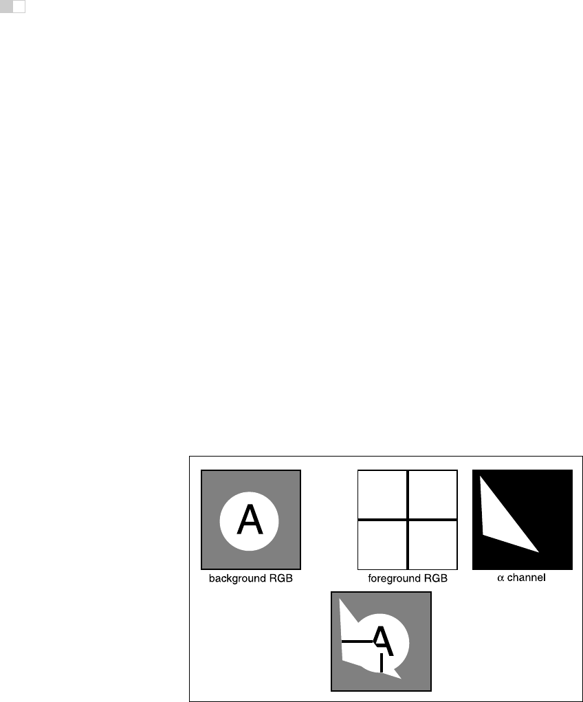
Figure 3.14. An example of compositing using Equation (3.2). The foreground image is
in effect cropped by the α channel before being put on top of the background image. The
resulting composite is shown on the bottom.
i
i
i
i
i
i
i
i
3.4. Alpha Compositing 67
3.4.1 Image Storage
Most RGB image formats use eight bits for each of the red, green, and blue chan-
nels. This results in approximately three megabytes of raw information for a sin-
gle million-pixel image. To reduce the storage requirement, most image formats
allow for some kind of compression. At a high level, such compression is ei-
ther lossless or lossy. No information is discarded in lossless compression, while
some information is lost unrecoverably in a lossy system. Popular image storage
formats include:
• jpeg. This lossy format compresses image blocks based on thresholds in
the human visual system. This format works well for natural images.
• tiff. This format is most commonly used to hold binary images or losslessly
compressed 8- or 16-bit RGB although many other options exist.
• ppm. This very simple lossless, uncompressed format is most often used
for 8-bit RGB images although many options exist.
• png. This is a set of lossless formats with a good set of open source man-
agement tools.
Because of compression and variants, writing input/output routines for images
can be involved. Fortunately one can usually rely on library routines to read and
write standard file formats. For quick-and-dirty applications, where simplicity is
valued above efficiency, a simple choice is to use raw ppm files, which can often
be written simply by dumping the array that stores the image in memory to a file,
prepending the appropriate header.
Frequently Asked Questions
• Why don’t they just make monitors linear and avoid all this gamma busi-
ness?
Ideally the 256 possible intensities of a monitor should look evenly spaced as op-
posed to being linearly spaced in energy. Because human perception of intensity is
itself non-linear, a gamma between 1.5 and 3 (depending on viewing conditions)
will make the intensities approximately uniform in a subjective sense. In this way
gamma is a feature. Otherwise the manufacturers would make the monitors linear.
..................Content has been hidden....................
You can't read the all page of ebook, please click here login for view all page.