

i
i
i
i
i
i
i
i
344 15. Curves
(a)
(b)
(c)
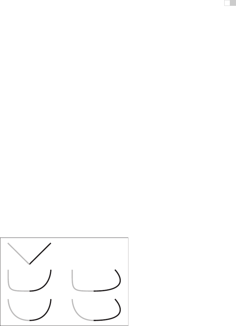
Figure 15.1. (a) A curve that can be easily represented as two lines; (b) a curve that can
be easily represented as a line and a circular arc; (c) a curve approximating curve (b) with
five line segments
For example, consider the curves in Figure 15.1. The first two curves are
easily specified in terms of two pieces. In the case of the curve in Figure 15.1(b),
we need two different kinds of pieces: a line segment and a circle.
To create a parametric representation of a compound curve (like the curve
in Figure 15.1(b)), we need to have our parametric function switch between the
functions that represent the pieces. If we define our parametric functions over the
range 0 ≤ u ≤ 1, then the curve in Figures 15.1(a) or (b) might be defined as
f(u)=
f
1
(2u)ifu ≤ 0.5,
f
2
(2u − 1) if u>0.5,
(15.2)
where f
1
is a parameterization of the first piece, f
2
is a parameterization of the
second piece, and both of these functions are defined over the unit interval.
We need to be careful in defining the functions f
1
and f
2
to make sure that the
pieces of the curve fit together. If f
1
(1) = f
2
(0), then our curve pieces will not
connect and will not form a single continuous curve.
To represent the curve in Figure 15.1(b), we needed to use two different types
of pieces: a line segment and a circular arc. For simplicity’s sake, we may prefer
to use a single type of piece. If we try to represent the curve in Figure 15.1(b)
with only one type of piece (line segments), we cannot exactly recreate the curve
(unless we use an infinite number of pieces). While the new curve made of line
segments (as in Figure 15.1(c)) may not be exactly the same shape as in Fig-
ure 15.1(b), it might be close enough for our use. In such a case, we might prefer
the simplicity of using the simpler line segment pieces to having a curve that more
accurately represents the shape.
Also, notice that as we use an increasing number of pieces, we can get a better
approximation. In the limit (using an infinite number of pieces), we can exactly
represent the original shape.
i
i
i
i
i
i
i
i
15.2. Curve Properties 345
One advantage to using a piecewise representation is that it allows us to make
a tradeoff between
1. how well our represented curve approximates the real shape we are trying
to represent;
2. how complicated the pieces that we use are;
3. how many pieces we use.
So, if we are trying to represent a complicated shape, we might decide that a
crude approximation is acceptable and use a small number of simple pieces. To
improve the approximation, we can choose between using more pieces and using
more complicated pieces.
In computer graphics practice, we tend to prefer using relatively simple curve
pieces (either line segments, arcs, or polynomial segments).
15.1.3 Splines
Before computers, when draftsmen wanted to draw a smooth curve, one tool they
employed was a stiff piece of metal that they would bend into the desired shape
for tracing. Because the metal would bend, not fold, it would have a smooth
shape. The stiffness meant that the metal would bend as little as possible to make
the desired shape. This stiff piece of metal was called a spline.
Mathematicians found that they could represent the curves created by a draft-
man’s spline with piecewise polynomial functions. Initially, they used the term
spline to mean a smooth, piecewise polynomial function. More recently, the term
spline has been used to describe any piecewise polynomial function. We prefer
this latter definition.
For us, a spline is a piecewise polynomial function. Such functions are very
useful for representing curves.
15.2 Curve Properties
To describe a curve, we need to give some facts about its properties. For “named”
curves, the properties are usually specific according to the type of curve. For
example, to describe a circle, we might provide its radius and the position of its
center. For an ellipse, we might also provide the orientation of its major axis and
the ratio of the lengths of the axes. For free-form curves however, we need to
have a more general set of properties to describe individual curves.
i
i
i
i
i
i
i
i
346 15. Curves
Some properties of curves are attributed to only a single location on the curve,
while other properties require knowledge of the whole curve. For an intuition of
the difference, imagine that the curve is a train track. If you are standing on the
track on a foggy day you can tell that the track is straight or curved and whether
or not you are at an end point. These are lo cal properties. You cannot tell whether
or not the track is a closed curve, or crosses itself, or how long it is. We call this
type of property, a global property.
The study of local properties of geometric objects (curves and surfaces) is
known as differential geometry. Technically, to be a differential property, there
are some mathematical restrictions about the properties (roughly speaking, in the
train-track analogy, you would not be able to have a GPS or a compass). Rather
than worry about this distinction, we will use the term local property rather than
differential property.
Local properties are important tools for describing curves because they do not
require knowledge about the whole curve. Local properties include
• continuity,
• position at a specificplaceonthecurve,
• direction at a specificplaceonthecurve,
• curvature (and other derivatives).
Often, we want to specify that a curve includes a particular point. A curve is
said to interpolate a point if that point is part of the curve. A function f interpo-
lates a value v if there is some value of the parameter u for which f (t)=v. We
call the place of interpolation, that is the value of t, the site.
15.2.1 Continuity
It will be very important to understand the local properties of a curve where two
parametric pieces come together. If a curve is defined using an equation like
Equation (15.2), then we need to be careful about how the pieces are defined. If
f
1
(1) = f
2
(0), then the curve will be “broken”—we would not be able to draw
the curve in a continuous stroke of a pen. We call the condition that the curve
pieces fit together continuity conditions because if they hold, the curve can be
drawn as a continuous piece. Because our definition of ”curve” at the beginning
of the chapter requires a curve to be continuous, technically a ”broken curve” is
not a curve.
i
i
i
i
i
i
i
i
15.2. Curve Properties 347
In addition to the positions, we can also check that the derivatives of the pieces
match correctly. If f
1
(1) = f
2
(0), then the combined curve will have an abrupt
change in its first derivative at the switching point; the first derivative will not
be continuous. In general, we say that a curve is C
n
continuous if all of its
derivatives up to n match across pieces. We denote the position itself as the
zeroth derivative, so that the C
0
continuity condition means that the positions
of the curve are continuous, and C
1
continuity means that positions and
first derivatives are continuous. The definition of curve requires the curve to
be C
0
.
An illustration of some continuity conditions is shown in Figure 15.2. A dis-
continuity in the first derivative (the curve is C
0
but not C
1
) is usually noticeable
because it displays a sharp corner. A discontinuity in the second derivative is
sometimes visually noticeable. Discontinuities in higher derivatives might mat-
ter, depending on the application. For example, if the curve represents a motion,
an abrupt change in the second derivative is noticeable, so third derivative con-
tinuity is often useful. If the curve is going to have a fluid flowing over it (for
example, if it is the shape for an airplane wing or boat hull), a discontinuity in the
fourth or fifth derivative might cause turbulence.
The type of continuity we have just introduced (C
n
) is commonly referred to
as parametric continuity as it depends on the parameterization of the two curve
pieces. If the “speed” of each piece is different, then they will not be continuous.
For cases where we care about the shape of the curve, and not its parameteriza-
tion, we define geometric continuity that requires that the derivatives of the curve
pieces match when the curves are parameterized equivalently (for example, us-
ing an arc-length parameterization). Intuitively, this means that the corresponding
derivatives must have the same direction, even if they have different magnitudes.
C
0
C
1
C
2
G
1
G
2
Figure 15.2. An illustration of various types of continuity between two curve segments.
i
i
i
i
i
i
i
i
348 15. Curves
So, if the C
1
continuity condition is
f
1
(1) = f
2
(0),
the G
1
continuity condition would be
f
1
(1) = k f
2
(0),
for some value of scalar k. Generally, geometric continuity is less restrictive
than parametric continuity. A C
n
curve is also G
n
except when the parametric
derivatives vanish.
15.3 Polynomial Pieces
The most widely used representations of curves in computer graphics is done
by piecing together basic elements that are defined by polynomials and called
polynomial pieces. For example, a line element is given by a linear polynomial.
In Section 15.3.1, we give a formal definition and explain how to put pieces of
polynomial together.
15.3.1 Polynomial Notation
Polynomials are functions of the form
f(t)=a
0
+ a
1
t + a
2
t
2
+ ...+ a
n
t
n
. (15.3)
The a
i
are called the coefficients. and n is called the degree of the polynomial if
a
n
=0. We also write Equation (15.3) in the form
f(t)=
n
i=0
a
i
t
i
. (15.4)
We call this the canonical form of the polynomial.
We can generalize the canonical form to
f(t)=
n
i=0
c
i
b
i
(t), (15.5)
where b
i
(t) is a polynomial. We can choose these polynomials in a convenient
form for different applications, and we call them basis functions or blending
functions (see Section 15.3.5). In Equation (15.4), the t
i
are the b
i
(t) of Equa-
tion (15.5). If the set of basis functions is chosen correctly, any polynomial of
degree n +1can be represented by an appropriate choice of c.
..................Content has been hidden....................
You can't read the all page of ebook, please click here login for view all page.