

i
i
i
i
i
i
i
i
2.5. Curves and Surfaces 33
where k
is any non-zero constant. By definition, “uphill” implies a positive
change in f, so we would like k
> 0,andk
=1is a perfectly good convention.
As an example of the gradient, consider the implicit circle x
2
+ y
2
− 1=
0 with gradient vector (2x, 2y), indicating that the outside of the circle is the
positive region for the function f (x, y)=x
2
+ y
2
− 1. Note that the length
of the gradient vector can be different depending on the multiplier in the implicit
equation. For example, the unit circle can be described by Ax
2
+Ay
2
−A =0for
any non-zero A. The gradient for this curve is (2Ax, 2Ay). This will be normal
(perpendicular) to the circle, but will have a length determined by A.ForA>0,
the normal will point outward from the circle, and for A<0, it will point inward.
This switch from outward to inward is as it should be, since the positive region
switches inside the circle. In terms of the height-field view, h = Ax
2
+ Ay
2
−A,
and the circle is at zero altitude. For A>0, the circle encloses a depression,
and for A<0, the circle encloses a bump. As A becomes more negative, the
Figure 2.27. The vector a
points in a direction where
f
has no change and is thus
perpendicular to the gradi-
ent vector ∇
f
.
bump increases in height, but the h =0circle doesn’t change. The direction
of maximum uphill doesn’t change, but the slope increases. The length of the
gradient reflects this change in degree of the slope. So intuitively, you can think
of the gradient’s direction as pointing uphill and its magnitude as measuring how
uphill the slope is.
Implicit 2D Lines
The familiar “slope-intercept” form of the line is
y = mx + b. (2.14)
This can be converted easily to implicit form (Figure 2.28):
y − mx − b =0. (2.15)
Here m is the “slope” (ratio of rise to run) and b is the y value where the line
crosses the y-axis, usually called the y-intercept . The line also partitions the 2D
plane, but here “inside” and “outside” might be more intuitively called “over” and
“under.”
Figure 2.28. A 2D line can
be described by the equa-
tion
y
−
mx
−
b
=0.
Because we can multiply an implicit equation by any constant without chang-
ing the points where it is zero, kf(x, y)=0is the same curve for any non-zero
k. This allows several implicit forms for the same line, for example,
2y − 2mx − 2b =0.
One reason the slope-intercept form is sometimes awkward is that it can’t rep-
resent some lines such as x =0because m would have to be infinite. For this

i
i
i
i
i
i
i
i
34 2. Miscellaneous Math
reason, a more general form is often useful:
Ax + By + C =0, (2.16)
for real numbers A, B, C.
Suppose we know two points on the line, (x
0
,y
0
) and (x
1
,y
1
).WhatA, B,
and C describe the line through these two points? Because these points lie on the
line, they must both satisfy Equation (2.16):
Ax
0
+ By
0
+ C =0,
Ax
1
+ By
1
+ C =0.
Unfortunately we have two equations and three unknowns: A, B,andC.This
problem arises because of the arbitrary multiplier we can have with an implicit
equation. We could set C =1for convenience:
Ax + By +1=0,
but we have a similar problem to the infinite slope case in slope-intercept form:
lines through the origin would need to have A(0) + B(0) + 1 = 0,whichisa
contradiction. For example, the equation for a 45-degree line through the origin
can be written x −y =0, or equally well y −x =0,oreven17y − 17x =0,but
it cannot be written in the form Ax + By +1=0.
Whenever we have such pesky algebraic problems, we try to solve the prob-
lems using geometric intuition as a guide. One tool we have, as discussed in
Section 2.5.2, is the gradient. For the line Ax + By + C =0, the gradient vector
is (A, B). This vector is perpendicular to the line (Figure 2.29), and points to the
Figure 2.29. The gradient
vector (
A, B
) is perpendi-
cular to the implicit line
Ax
+
By
+
C
=0.
side of the line where Ax + By + C is positive. Given two points on the line
(x
0
,y
0
) and (x
1
,y
1
), we know that the vector between them points in the same
direction as the line. This vector is just (x
1
−x
0
,y
1
−y
0
), and because it is paral-
lel to the line, it must also be perpendicular to the gradient vector (A, B). Recall
that there are an infinite number of (A, B, C) that describe the line because of the
arbitrary scaling property of implicits. We want any one of the valid (A, B, C).
We can start with any (A, B) perpendicularto (x
1
−x
0
,y
1
−y
0
). Such a vector
is just (A, B)=(y
0
− y
1
,x
1
− x
0
) by the same reasoning as in Section 2.5.2.
This means that the equation of the line through (x
0
,y
0
) and (x
1
,y
1
) is
(y
0
− y
1
)x +(x
1
− x
0
)y + C =0. (2.17)
Now we just need to find C. Because (x
0
,y
0
) and (x
1
,y
1
) are on the line, they
must satisfy Equation (2.17). We can plug either value in and solve for C. Doing
this for (x
0
,y
0
) yields C = x
0
y
1
−x
1
y
0
, and thus the full equation for the line is
(y
0
− y
1
)x +(x
1
− x
0
)y + x
0
y
1
− x
1
y
0
=0. (2.18)
i
i
i
i
i
i
i
i
2.5. Curves and Surfaces 35
Again, this is one of infinitely many valid implicit equations for the line through
two points, but this form has no division operation and thus no numerically de-
generate cases for points with finite Cartesian coordinates. A nice thing about
Equation (2.18) is that we can always convert to the slope-intercept form (when
it exists) by moving the non-y terms to the right-hand side of the equation and
dividing by the multiplier of the y term:
y =
y
1
− y
0
x
1
− x
0
x +
x
1
y
0
− x
0
y
1
x
1
− x
0
.
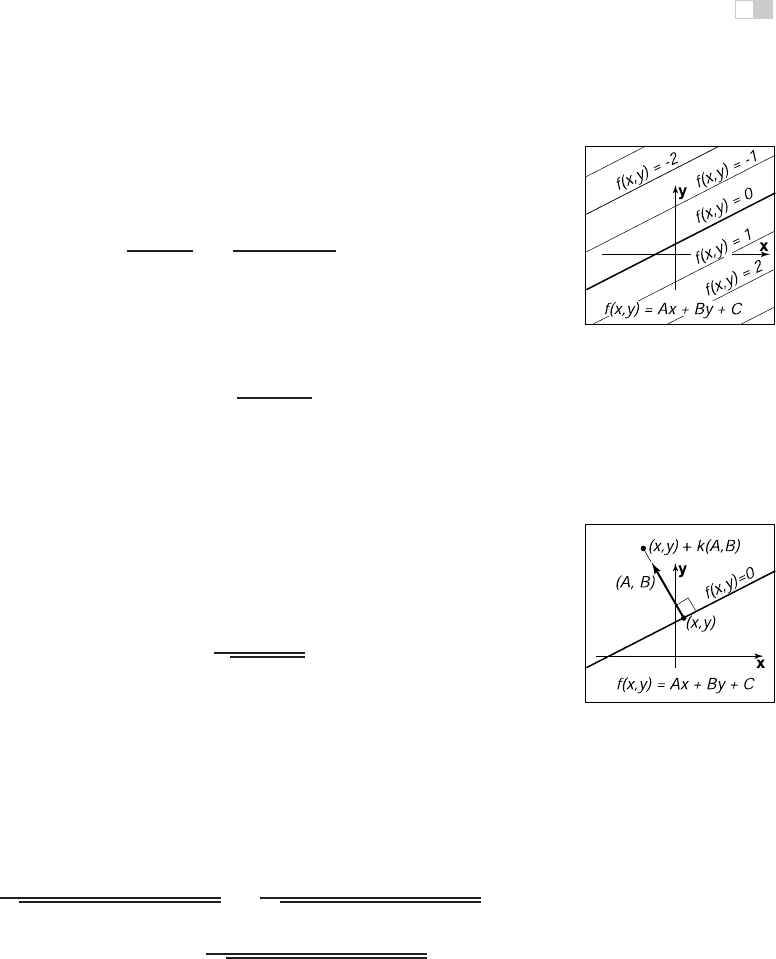
An interesting property of the implicit line equation is that it can be used to find
the signed distance from a point to the line. The value of Ax + By + C is
Figure 2.30. The value
of the implicit function
f
(
x,y
)
=
Ax
+
By
+
C
is a con-
stant times the signed dis-
tance from
Ax
+
By
+
C
=0.
proportional to the distance from the line (Figure 2.30). As shown in Figure 2.31,
the distance from a point to the line is the length of the vector k(A, B),whichis
distance = k
A
2
+ B
2
. (2.19)
For the point (x, y)+k(A, B),thevalueoff(x, y)=Ax + By + C is
f(x + kA, y + kB)=Ax + kA
2
+ By + kB
2
+ C
= k(A
2
+ B
2
).
(2.20)
The simplification in that equation is a result of the fact that we know (x, y) is on
the line, so Ax + By + C =0. From Equations (2.19) and (2.20), we can see that
the signed distance from line Ax + By + C =0to a point (a, b) is
distance =
f(a, b)
√
A
2
+ B
2
.
Here “signed distance” means that its magnitude (absolute value) is the geometric
Figure 2.31. The vec-
tor
k
(
A,B
) connects a point
(
x,y
) on the line closest to
a point not on the line.
The distance is proportional
to
k
.
distance, but on one side of the line, distances are positiveand on the other they are
negative. You can choose between the equally valid representations f(x, y)=0
and −f(x, y)=0if your problem has some reason to prefer a particular side
being positive. Note that if (A, B) is a unit vector, then f(a, b) is the signed
distance. We can multiply Equation (2.18) by a constant that ensures that (A, B)
is a unit vector:
f(x, y)=
y
0
− y
1
(x
1
− x
0
)
2
+(y
0
− y
1
)
2
x +
x
1
− x
0
(x
1
− x
0
)
2
+(y
0
− y
1
)
2
y
+
x
0
y
1
− x
1
y
0
(x
1
− x
0
)
2
+(y
0
− y
1
)
2
=0. (2.21)
Note that evaluating f (x, y) in Equation (2.21) directly gives the signed distance,
but it does require a square root to set up the equation. Implicit lines will turn
out to be very useful for triangle rasterization (Section 8.1.2). Other forms for 2D
lines are discussed in Chapter 14.

i
i
i
i
i
i
i
i
36 2. Miscellaneous Math
Implicit Quadric Curves
In the previous section we saw that a linear function f(x, y) gives rise to an im-
plicit line f(x, y)=0.Iff is instead a quadratic function of x and y, with the
general form
Ax
2
+ Bxy + Cy
2
+ Dx + Ey + F =0,
the resulting implicit curve is called a quadric. Two-dimensional quadric curves
Figure 2.32. The ellipse
with center (
x
c
,y
c
) and
semi-axes of length
a
and
b
.
include ellipses and hyperbolas, as well as the special cases of parabolas, circles,
and lines.
Examples of quadric curves include the circle with center (x
c
,y
c
) and ra-
dius r:
(x − x
c
)
2
+(y − y
c
)
2
− r
2
=0
where (x
c
,y
c
) is the center of the ellipse, and a and b are the minor and majorTry setting
a=b=r
in the
ellipse equation and com-
pare to the circle equation.
semi-axes (Figure 2.32).and axis-aligned ellipses of the form
(x − x
c
)
2
a
2
+
(y − y
c
)
2
b
2
− 1=0.
2.5.3 3D Implicit Surfaces
Just as implicit equations can be used to define curves in 2D, they can be used to
define surfaces in 3D. As in 2D, implicit equations implicitly define a set of points
that are on the surface
f(x, y, z)=0.
Any point (x, y, z) that is on the surface results in zero when given as an argument
to f. Any point not on the surface results in some number other than zero. You
can check whether a point is on the surface by evaluating f, or you can check
which side of the surface the point lies on by looking at the sign of f , but you
cannot always explicitly construct points on the surface. Using vector notation,
we will write such functions of p =(x, y, z) as
f(p)=0.
2.5.4 Surface Normal to an Implicit Surface
A surface normal (which is needed for lighting computations, among other things)
is a vector perpendicular to the surface. Each point on the surface may have a
different normal vector. In the same way that the gradient provides a normal to

i
i
i
i
i
i
i
i
2.5. Curves and Surfaces 37
an implicit curve in 2D, the surface normal at a point p on an implicit surface is
given by the gradient of the implicit function
n = ∇f(p)=
∂f(p)
∂x
,
∂f(p)
∂y
,
∂f(p)
∂z
.
The reasoning is the same as for the 2D case: the gradient points in the direction
of fastest increase in f , which is perpendicular to the direction’s tangent to the
surface, in which f remains constant. The gradient vector points toward the side
of the surface where f(p) > 0, which we may think of as “into” the surface or
“out from” the surface in a given context. If the particular formof f creates inward
facing gradients and outward facing gradients are desired, the surface −f(p)=0
is the same as surface f (p)=0but has directionally reversed gradients, i.e.,
−∇f(p)=∇(−f (p)).
2.5.5 Implicit Planes
As an example, consider the infinite plane through point a with surface normal n.
The implicit equation to describe this plane is given by
(p − a) · n =0. (2.22)
Note that a and n are known quantities. The point p is any unknown point that
satisfies the equation. In geometric terms this equation says “the vector from a to
p is perpendicular to the plane normal.” If p were not in the plane, then (p − a)
would not make a right angle with n (Figure 2.33).
Figure 2.33. Any of the
points p shown are in the
plane with normal vector
n that includes point a if
Equation (2.2) is satisfied.
Sometimes we want the implicit equation for a plane through points a, b,
and c. The normal to this plane can be found by taking the cross product of any
two vectors in the plane. One such cross product is
n =(b − a) × (c − a).
This allows us to write the implicit plane equation:
(p − a) · ((b − a) × (c − a)) = 0. (2.23)
A geometric way to read this equation is that the volume of the parallelepiped
defined by p − a, b − a,andc − a is zero, i.e., they are coplanar. This can
only be true if p is in the same plane as a, b,andc. The full-blown Cartesian
representation for this is given by the determinant (this is discussed in more detail
in Section 5.3):
x − x
a
y − y
a
z − z
a
x
b
− x
a
y
b
− y
a
z
b
− z
a
x
c
− x
a
y
c
− y
a
z
c
− z
a
=0. (2.24)
..................Content has been hidden....................
You can't read the all page of ebook, please click here login for view all page.