

i
i
i
i
i
i
i
i
38 2. Miscellaneous Math
The determinant can be expanded (see Section 5.3 for the mechanics of expanding
determinants) to the bloated form with many terms.
Equations (2.23) and (2.24) are equivalent, and comparing them is instruc-
tive. Equation (2.23) is easy to interpret geometrically and will yield efficient
code. In addition, it is relatively easy to avoid a typographic error that compiles
into incorrect code if it takes advantage of debugged cross and dot product code.
Equation (2.24) is also easy to interpret geometrically and will be efficient pro-
vided an efficient 3 × 3 determinant function is implemented. It is also easy to
implement without a typo if a function determinant(a, b, c) is available. It will
be especially easy for others to read your code if you rename the determinant
function volume. So both Equations (2.23) and (2.24) map well into code. The
full expansion of either equation into x-, y-, and z-components is likely to gener-
ate typos. Such typos are likely to compile and, thus, be especially pesky. This
is an excellent example of clean math generating clean code and bloated math
generating bloated code.
3D Quadric Surfaces
Just as quadraticpolynomialsin two variablesdefine quadric curves in 2D, quadratic
polynomials in x, y,andz define quadric surfaces in 3D. For instance, a sphere
can be written as
f(p)=(p −c)
2
− r
2
=0,
and an axis-aligned ellipsoid may be written as
f(p)=
(x − x
c
)
2
a
2
+
(y − y
c
)
2
b
2
+
(z − z
c
)
2
c
2
− 1=0.
3D Curves from Implicit Surfaces
One might hope that an implicit 3D curve could be created with the form f(p)=
0. However, all such curves are just degenerate surfaces and are rarely useful in
practice. A 3D curvecan be constructedfrom the intersection of two simultaneous
implicit equations:
f(p)=0,
g(p)=0.
For example, a 3D line can be formed from the intersection of two implicit planes.
Typically, it is more convenient to use parametric curves instead; they are dis-
cussed in the following sections.
i
i
i
i
i
i
i
i
2.5. Curves and Surfaces 39
2.5.6 2D Parametric Curves
A parametric curve is controlled by a single parameter that can be considered a
sort of index that moves continuously along the curve. Such curves have the form
x
y
=
g(t)
h(t)
.
Here (x, y) is a point on the curve, and t is the parameter that influences the curve.
For a given t, there will be some point determined by the functions g and h.For
continuous g and h, a small change in t will yield a small change in x and y.
Thus, as t continuously changes, points are swept out in a continuous curve. This
is a nice feature because we can use the parameter t to explicitly construct points
on the curve. Often we can write a parametric curve in vector form,
p = f(t),
where f is a vector-valued function, f : R → R
2
. Such vector functions can
generate very clean code, so they should be used when possible.
We can think of the curve with a position as a function of time. The curve
can go anywhere and could loop and cross itself. We can also think of the curve
as having a velocity at any point. For example, the point p(t) is traveling slowly
near t = −2 and quickly between t =2and t =3. This type of “moving point”
vocabulary is often used when discussing parametric curves even when the curve
is not describing a moving point.
2D Parametric Lines
A parametric line in 2D that passes through points p
0
=(x
0
,y
0
) and p
1
=
(x
1
,y
1
) can be written
x
y
=
x
0
+ t(x
1
− x
0
)
y
0
+ t(y
1
− y
0
)
.
Because the formulas for x and y have such similar structure, we can use the
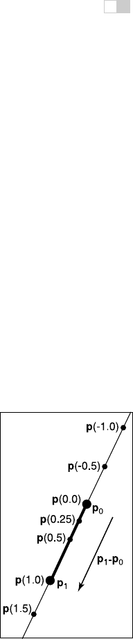
vector form for p =(x, y) (Figure 2.34):
Figure 2.34. A 2D para-
metric line through p
0
and
p
1
. The line segment de-
fined by
t
∈ [0,1] is shown
in bold.
p(t)=p
0
+ t(p
1
− p
0
).
You can read this in geometric form as: “start at point p
0
and go some distance
toward p
1
determined by the parameter t.” A nice feature of this form is that
p(0) = p
0
and p(1) = p
1
. Since the point changes linearly with t,thevalueof
t between p
0
and p
1
measures the fractional distance between the points. Points
i
i
i
i
i
i
i
i
40 2. Miscellaneous Math
with t<0 are to the “far” side of p
0
, and points with t>1 are to the “far” side
of p
1
.
Parametric lines can also be described as just a point o and a vector d:
p(t)=o + t(d).
When the vector d has unit length, the line is arc-length parameterized.This
means t is an exact measure of distance along the line. Any parametric curve can
be arc-length parameterized, which is obviously a very convenient form, but not
all can be converted analytically.
2D Parametric Circles
A circle with center (x
c
,y
c
) and radius r has a parametric form:
x
y
=
x
c
+ r cos φ
y
c
+ r sin φ
.
To ensure that there is a unique parameter φ for every point on the curve, we can
restrict its domain: φ ∈ [0, 2π) or φ ∈ (−π, π] or any other half open interval of
length 2π.
An axis-aligned ellipse can be constructed by scaling the x and y parametric
equations separately:
x
y
=
x
c
+ a cos φ
y
c
+ b sin φ
.
2.5.7 3D Parametric Curves
A 3D parametric curve operates much like a 2D parametric curve:
x = f (t),
y = g(t),
z = h(t).
For example, a spiral around the z-axis is written as:
x =cost,
y =sint,
z = t.
i
i
i
i
i
i
i
i
2.5. Curves and Surfaces 41
As with 2D curves, the functions f, g,andh are defined on a domain D ⊂ R if
we want to control where the curve starts and ends. In vector form we can write
⎡
⎣
x
y
z
⎤
⎦
= p(t).
The parametric curve is the
range of p: R → R
3
.
In this chapter we only discuss 3D parametric lines in detail. General 3D
parametric curves are discussed more extensively in Chapter 15.
3D Parametric Lines
A 3D parametric line can be written as a straightforward extension of the 2D
parametric line, e.g.,
x =2+7t,
y =1+2t,
z =3−5t.
This is cumbersome and does not translate well to code variables, so we will write
it in vector form:
p = o + td,
where, for this example, o and d are given by
o =(2, 1, 3),
d =(7, 2, −5).
Note that this is very similar to the 2D case. The way to visualize this is to
imagine that the line passes though o and is parallel to d. Given any value of t,
you get some point p(t) on the line. For example, at t =2, p(t)=(2, 1, 3) +
2(7, 2, −5) = (16, 5, −7). This general concept is the same as for two dimensions
(Figure 2.30).
As in 2D, a line segment can be described by a 3D parametric line and an
interval t ∈ [t
a
,t
b
]. The line segment between two points a and b is given by
p(t)=a + t(b − a) with t ∈ [0, 1].Herep(0) = a, p(1) = b,andp(0.5) =
(a + b)/2, the midpoint between a and b.
A ray,orhalf-line, is a 3D parametric line with a half-open interval, usu-
ally [0, ∞). From now on we will refer to all lines, line segments, and rays
as “rays.” This is sloppy, but corresponds to common usage and makes the
discussion simpler.

i
i
i
i
i
i
i
i
42 2. Miscellaneous Math
2.5.8 3D Parametric Surfaces
The parametric approach can be used to define surfaces in 3D space in much the
same way we define curves, except that there are two parameters to address the
two-dimensional area of the surface. These surfaces have the form
x = f(u, v),
y = g(u, v),
z = h(u, v).
or, in vector form,
The parametric surface is
the range of the function p:
R
2
→ R
3
.
⎡
⎣
x
y
z
⎤
⎦
= p(u, v).
Example. For example, a point on the surface of the Earth can be described by thePretend for the sake of ar-
gument that the Earth is ex-
actly spherical.
two parameters longitude and latitude. If we define the origin to be at the center of
the earth, and let r be the radius of the Earth, then a spherical coordinate system
centered at the origin (Figure 2.35), lets us derive the parametric equations
The θ and φ here may
or may not seem reversed
depending on your back-
ground; the use of these
symbols varies across dis-
ciplines. In this book we will
always assume the mean-
ing of
θ and φ used in
Equation (2.25) and de-
picted in Figure 2.35.
x = r cos φ sin θ,
y = r sin φ sin θ,
z = r cos θ.
(2.25)
Ideally, we’d like to write this in vector form, but it isn’t feasible for this particular
parametric form.
We would also like to be able to find the (θ, φ) for a given (x, y, z).Ifwe
assume that φ ∈ (−π, π] this is easy to do using the atan2 function from Equa-
tion (2.2):
θ = acos(z/
x
2
+ y
2
+ z
2
),
φ = atan2(y,x).
(2.26)
With implicit surfaces, the derivative of the function f gave us the surface
normal. With parametric surfaces, the derivatives of p also give information about
the surface geometry.
Figure 2.35. The ge-
ometry for spherical coordi-
nates.
Consider the function q(t)=p(t, v
0
). This function defines a parametric
curve obtained by varying u while holding v fixed at the value v
0
. This curve,
called an isoparametric curve (or sometimes “isoparm” for short) lies in the sur-
face. The derivative of q gives a vector tangent to the curve, and since the curve
..................Content has been hidden....................
You can't read the all page of ebook, please click here login for view all page.