
i
i
i
i
i
i
i
i
17.2. Keyframing 423
slope of s(t) gives the velocity of motion with negative slope corresponding to
the motion backwards along the curve. To achieve most flexibility, the ability to
interactively edit s(t) is typically provided to the animator by the animation sys-
tem. The distance-time function is not the only way to control motion. In some
cases it might be more convenient for the user to specify a velocity-time function
v(t) or even an acceleration-time function a(t). Since these are correspondingly
first and second derivatives of s(t), to use these type of controls, the system first
recovers the distance-time function by integrating the user input (twice in the case
of a(t)).
The relationship between the curve parameter u and arc length s is established
automatically by the system. In practice, the system first determines arc length
dependance on parameter u (i.e., the inverse function s(u)). Using this function,
for any given S it is possible to solve the equation s(u) −S =0with unknown u
obtaining u(S). For most curves, the function s(u) can not be expressed in closed
analytic form and numerical integration is necessary (see Chapter 14). Standard
numerical root-finding procedures (such as the Newton-Raphson method, for ex-
ample) can then be directly used to solve the equation s(u) − S =0for u.
u=0.8
u=0.4
u=0.6
u=1.0
u=0
u=0.2
s(u)
u
0.2
0.4
1.0
0.8
0.6
0.0
2.5
8.5
7.0
5.0
4.0
0.0
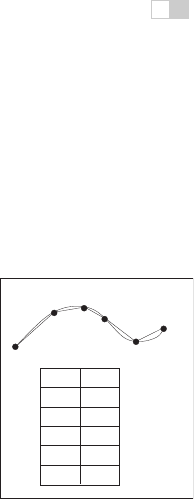
Figure 17.9. To cre-
ate a tabular version of
s
(
u
), the curve can be ap-
proximated by a number
of line segments connect-
ing points on the curve po-
sitioned at equal parame-
ter increments. The table
is searched to find the
u
-
interval for a given
S
.For
the curve above, for exam-
ple, the value of
u
corre-
sponding to the position of
S
= 6.5 lies between
u
=0.6
and
u
=0.8.
An alternative technique is to approximate the curve itself as a set of linear
segments between points p
i
computed at some set of sufficiently densely spaced
parameter values u
i
. One then creates a table of approximate arc lengths
s(u
i
) ≈
i
j=1
||p
j
− p
j−1
|| = s(u
i−1
)+||p
i
− p
i−1
||.
Since s(u) is a non-decreasing function of u, one can then find the interval con-
taining the value S by simple searching through the table (see Figure17.9). Linear
interpolation of the interval’s u end values is then performed to finally find u(S).
If greater precision is necessary, a few steps of the Newton-Raphson algorithm
with this value as the starting point can be applied.
17.2.2 Interpolating Rotation
The techniques presented above can be used to interpolate the keys set for most of
the parameters describing the scene. Three-dimensional rotation is one important
motion for which more specialized interpolation methods and representations are
common. The reason for this is that applying standard techniques to 3D rotations
often leads to serious practical problems. Rotation (a change in orientation of an
object) is the only motion other than translation which leaves the shape of the
object intact. It therefore plays a special role in animating rigid objects.
i
i
i
i
i
i
i
i
424 17. Computer Animation
X
Y
Y
Z
X
Z
Y
Y
X
Z
X
Z
rotate(X)
rotate(Z)
rotate(Y)
Figure 17.10. Three Euler angles can be used to specify arbitrary object orientation through
a sequence of three rotations around coordinate axes embedded into the object (axis Y
always points to the tip of the cone). Note that each rotation is given in a new coordinate
system. Fixed angle representation is very similar but the coordinate axes it uses are fixed
in space and do not rotate with the object.
There are several ways to specify the orientation of an object. First, trans-
formation matrices as described in Chapter 6 can be used. Unfortunately, naive
(element-by-element)interpolation of rotation matrices does not produce a correct
result. For example, the matrix “half-way” between 2D clock- and counterclock-
wise 90 degree rotation is the null matrix:
1
2
01
−10
+
1
2
0 −1
10
=
00
00
.
The correct result is, of course, the unit matrix corresponding to no rotation. Sec-
ond, one can specify arbitrary orientation as a sequence of exactly three rotations
around coordinate axes chosen in some specific order. These axes can be fixed in
space (fixed-angle representation) or embedded into the object therefore changing
after each rotation (Euler-angle representation as shown in Figure 17.10). These
three angles of rotation can be animated directly through standard keyframing,
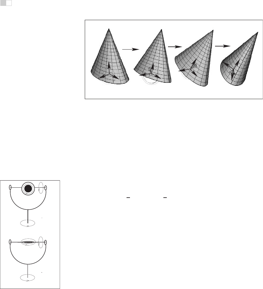
but a subtle problem known as gimbal lock arises. Gimbal lock occurs if dur-
ing rotation one of the three rotation axes is by accident aligned with another,
thereby reducing by one the number of available degrees of freedom as shown in
Figure 17.11 for a physical device. This effect is more common than one might
rotate(X)
rotate(Z)
rotate(Y)
Original configuration
rotate(Z)
rotate(Y)
rotate(X)
Gimbal lock configuration
Figure 17.11. In this
example, gimbal lock oc-
curs when a 90 degree
turn around axis Z is made.
Both X and Y rotations are
now performed around the
same axis leading to the
loss of one degree of free-
dom.
think—a single 90 degree turn to the right (or left) can potentially put an object
into a gimbal lock. Finally, any orientation can be specified by choosing an appro-
priate axis in space and angle of rotation around this axis. While animating in this
representation is relatively straightforward, combining two rotations, i.e., finding
the axis and angle corresponding to a sequence of two rotations both represented
by axis and angle, is non-trivial. A special mathematical apparatus, quaternions

i
i
i
i
i
i
i
i
17.2. Keyframing 425
has been developed to make this representation suitable both for combining sev-
eral rotations into a single one and for animation.
Given a 3D vector v =(x, y, z) and a scalar s, a quaternion q is formed by
combining the two into a four component object: q =[sxyz]=[s; v]. Several
new operations are then defined for quaternions. Quaternion addition simply sums
scalar and vector parts separately:
q
1
+ q
2
≡ [s
1
+ s
2
; v
1
+ v
2
].
Multiplication by a scalar a gives a new quaternion
aq ≡ [as; av].
More complex quaternion multiplication is defined as
q
1
·q
2
≡ [s
1
s
2
− v
1
v
2
; s
1
v
2
+ s
2
v
1
+ v
1
× v
2
],
where × denotes a vector cross product. It is easy to see that, similar to matrices,
quaternion multiplication is associative, but not commutative. We will be inter-
ested mostly in normalized quaternions—those for which the quaternion norm
|q| =
√
s
2
+ v
2
is equal to one. One final definition we need is that of an inverse
quaternion:
q
−1
=(1/|q|)[s; −v].
To represent a rotation by angle φ around an axis passing through the origin
whose direction is given by the normalized vector n, a normalized quaternion
q =[cos(φ/2); sin(φ/2)n]
is formed. To rotate point p, one turns it into the quaternion q
p
=[0; p] and
q2
q1
Figure 17.12. Inter-
polating quaternions should
be done on the surface of
a 3D unit sphere embed-
ded in 4D space. How-
ever, much simpler interpo-
lation along a 4D straight
line (open circles) followed
by re-projection of the re-
sults onto the sphere (black
circles) is often sufficient.
computes the quaternion product
q
p
= q · q
p
·q
−1
which is guaranteed to have a zero scalar part and the rotated point as its vector
part. Composite rotation is given simply by the product of quaternions represent-
ing each of the separate rotation steps. To animate with quaternions, one can treat
them as points in a four-dimensional space and set keys directly in this space. To
keep quaternions normalized, one should, strictly speaking, restrict interpolation
procedures to a unit sphere (a 3D object) in this 4D space. However, a spherical
version of even linear interpolation (often called slerp) already results in rather
unpleasant math. Simple 4D linear interpolation followed by projection onto the
unit sphere shown in Figure 17.12 is much simpler and often sufficient in practice.
Smoother results can be obtained via repeated application of a linear interpolation
procedure using the de Casteljau algorithm.
i
i
i
i
i
i
i
i
426 17. Computer Animation
17.3 Deformations
Although techniques for object deformation might be more properly treated as
modeling tools, they are traditionally discussed together with animation methods.
Probably the simplest example of an operation which changes object shape is a
non-uniform scaling. More generally, some function can be applied to local co-
ordinates of all points specifying the object (i.e., vertices of a triangular mesh
or control polygon of a spline surface), repositioning these points and creating a
new shape: p
= f(p,γ) where γ is a vector of parameters used by the deforma-
tion function. Choosing different f (and combining them by applying one after
another) can help to create very interesting deformations. Examples of useful
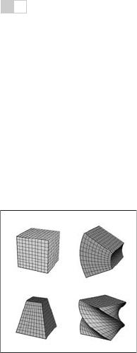
simple functions include bend, twist, and taper which are shown in Figure 17.13.
Animating shape change is very easy in this case by keyframing the parameters
of the deformation function. Disadvantages of this technique include difficulty of
choosing the mathematical function for some non-standard deformations and the
fact that the resulting deformation is global in the sense that the complete object,
and not just some part of it, is reshaped.
BendOriginal shape
Taper
Twist
Figure 17.13. Popular ex-
amples of global deforma-
tions. Bending and twist an-
gles as well as the degree
of taper can all be animated
to achieve dynamic shape
change.
To deform an object locally while providing more direct control over the re-
sult, one can choose a single vertex, move it to a new location and adjust vertices
within some neighborhood to follow the seed vertex. The area affected by the de-
formation and the specific amount of displacement in different parts of the object
are controlled by an attenuation function which decreases with distance (typically
computed over the object’s surface) to the seed vertex. Seed vertex motion can be
keyframed to produce animated shape change.
A more general deformation technique is called free-form deformation (FFD)
(Sederberg & Parry, 1986). A local (in most cases rectilinear) coordinate grid
is first established to encapsulate the part of the object to be deformed, and co-
ordinates (s, t, u) of all relevant points are computed with respect to this grid.
The user then freely reshapes the grid of lattice points P
ijk
into a new distorted
lattice P
ijk
(Figure 17.14). The object is reconstructed using coordinates com-
puted in the original undistorted grid in the trivariate analog of B´ezier interpolants
(see Chapter 15) with distorted lattice points P
ijk
serving as control points in this
expression:
P (s, u, t)=
L
i=0
i
L
(1 − s)
L−i
s
i
M
j=0
j
M
(1 − t)
M−j
t
j
N
k=0
k
N
(1 − u)
N−k
u
k
P
ijk
,
where L, M, N are maximum indices of lattice points in each dimension. In ef-
fect, the lattice serves as a low resolution version of the object for the purpose of
deformation, allowing for a smooth shape change of an arbitrarily complex ob-
i
i
i
i
i
i
i
i
17.4. Character Animation 427
ject through a relatively small number of intuitive adjustments. FFD lattices can
themselves be treated as regular objects by the system and can be transformed, an-
imated, and even further deformed if necessary, leading to corresponding changes
in the object to which the lattice is attached. For example, moving a deforma-
tion tool consisting of the original lattice and distorted lattice representing a bulge
across an object results in a bulge moving across the object.
Figure 17.14. Adjusting
the FFD lattice results in the
deformation of the object.
17.4 Character Animation
Animation of articulated figures is most often performed through a combination
of keyframing and specialized deformation techniques. The character model in-
tended for animation typically consists of at least two main layers as shown in
Figure 17.15. The motion of a highly detailed surface representing the outer shell
or skin of the character is what the viewer will eventually see in the final prod-
uct. The skeleton underneath it is a hierarchical structure (a tree) of joints which
provides a kinematic model of the figure and is used exclusively for animation.
In some cases, additional intermediate layer(s) roughly corresponding to muscles
are inserted between the skeleton and the skin.
skeleton
skin
Figure 17.15. (Left) A hierarchy of joints, a skeleton, serves as a kinematic abstraction of
the character; (middle) repositioning the skeleton deforms a separate skin object attached
to it; (right) a tree data structure is used to represent the skeleton. For compactness, the
internal structure of several nodes is hidden (they are identical to a corresponding sibling).
..................Content has been hidden....................
You can't read the all page of ebook, please click here login for view all page.