
i
i
i
i
i
i
i
i
228 9. Signal Processing
originalsampledsampled × 2sampled × 4
T
T
1
T
T
1
T
T
1
aliasing
aliasing
minimal
aliasing
x u
0
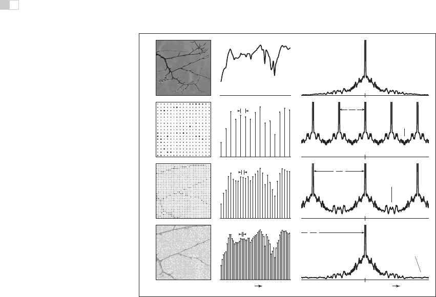
Figure 9.49. The effect of sample rate on the frequency spectrum of the sampled signal.
Higher sample rates push the copies of the spectrum apart, reducing problems caused by
overlap.
The key criterion is that the width of the spectrum must be less than the dis-
tance between the copies—that is, the highest frequency present in the signal
must be less than half the sample frequency. This is known as the Nyquist crite-
rion, and the highest allowable frequency is known as the Nyquist frequency or
Nyquist limit.TheNyquist-Shannon sampling theorem states that a signal whose
frequencies do not exceed the Nyquist limit (or, said another way, a signal that is
bandlimited to the Nyquist frequency) can, in principle, be reconstructed exactly
from samples.
With a high enough sample rate for a particular signal, we don’t need to use
a sampling filter. But if we are stuck with a signal that contains a wide range of
frequencies (such as an image with sharp edges in it), we must use a sampling
filter to bandlimit the signal before we can sample it. Figure 9.50 shows the
effects of three lowpass (smoothing) filters in the frequency domain, and Figure
9.51 shows the effect of using these same filters when sampling. Even if the
spectra overlap without filtering, convolving the signal with a lowpass filter can
narrow the spectrum enough to eliminate overlap and produce a well-sampled
i
i
i
i
i
i
i
i
9.5. Sampling Theory 229
1
originalmild blurstrong blur
x u
0
filter
filter
1
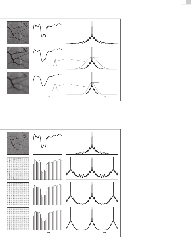
Figure 9.50. Applying lowpass (smoothing) filters narrows the frequency spectrum of a
signal.
originalsamp.: no filtersamp.: mild blursamp.: strong blur
x u0
severe
aliasing
some
aliasing
minimal
aliasing
Figure 9.51. How the lowpass filters from Figure 9.50 prevent aliasing during sampling.
Lowpass filtering narrows the spectrum so that the copies overlap less, and the high fre-
quencies from the alias spectra interfere less with the base spectrum.
i
i
i
i
i
i
i
i
230 9. Signal Processing
1
1
1
originalbox recon.tent recon.B-spline recon.
x u0
filter
filter
filter
severe
aliasing
some
aliasing
minimal
aliasing
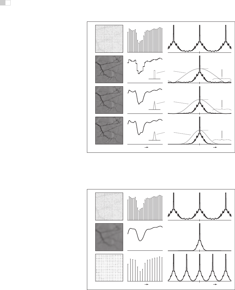
Figure 9.52. The effects of different reconstruction filters in the frequency domain. A
good reconstruction filter attenuates the alias spectra effectively while preserving the base
spectrum.
originalreconstructedresampled
x u
0
Figure 9.53. Resampling viewed in the frequency domain. The resampling filter both
reconstructs the signal (removes the alias spectra) and bandlimits it (reduces its width) for
sampling at the new rate.
i
i
i
i
i
i
i
i
9.5. Sampling Theory 231
representation of the filtered signal. Of course, we have lost the high frequencies,
but that’s better than having them get scrambled with the signal and turn into
artifacts.
Preventing Aliasing in Reconstruction
From the frequency domain perspective, the job of a reconstruction filter is to re-
move the alias spectra while preserving the base spectrum. In Figure 9.48, we can
see that the crudest reconstruction filter, the box, does attenuate the alias spec-
tra. Most important, it completely blocks the DC spike for all the alias spectra.
This is a characteristic of all reasonable reconstruction filters: they have zeroes
in frequency space at all multiples of the sample frequency. This turns out to be
equivalent to the ripple-free property in the space domain.
So a good reconstruction filter needs to be a good lowpass filter, with the
added requirement of completely blocking all multiples of the sample frequency.
The purpose of using a reconstruction filter different from the box filter is to more
completely eliminate the alias spectra, reducing the leakage of high-frequency ar-
tifacts into the reconstructed signal, while disturbing the base spectrum as little
as possible. Figure 9.52 illustrates the effects of different filters when used dur-
ing reconstruction. As we have seen, the box filter is quite “leaky” and results in
plenty of artifacts even if the sample rate is high enough. The tent filter, result-
ing in linear interpolation, attenuates high frequencies more, resulting in milder
artifacts, and the B-spline filter is very smooth, controlling the alias spectra very
effectively. It also smooths the base spectrum some—this is the tradeoff between
smoothing and aliasing that we saw earlier.
Preventing Aliasing in Resampling
When the operations of reconstruction and sampling are combined in resampling,
the same principles apply, but with one filter doing the work of both reconstruction
and sampling. Figure 9.53 illustrates how a resampling filter must remove the
alias spectra and leave the spectrum narrow enough to be sampled at the new
sample rate.
9.5.6 Ideal Filters vs. Useful Filters
Following the frequency domain analysis to its logical conclusion, a filter that is
exactly a box in the frequency domain is ideal for both sampling and reconstruc-
tion. Such a filter would prevent aliasing at both stages without diminishing the
frequencies below the Nyquist frequency at all.
i
i
i
i
i
i
i
i
232 9. Signal Processing
Recall that the inverse and forward Fourier transforms are essentially iden-
tical, so the spatial domain filter that has a box as its Fourier transform is the
function sin πx/πx = sinc πx.
However, the sinc filter is not generally used in practice, either for sampling or
for reconstruction, because it is impractical and because, even though it is optimal
according to the frequency domain criteria, it doesn’t produce the best results for
many applications.
For sampling, the infinite extent of the sinc filter, and its relatively slow rate
of decrease with distance from the center, is a liability. Also, for some kinds of
sampling, the negative lobes are problematic. A Gaussian filter makes an excel-
lent sampling filter even for difficult cases where high-frequency patterns must be
removed from the input signal, because its Fourier transform falls off exponen-
tially, with no bumps that tend to let aliases leak through. For less difficult cases,
atentfilter generally suffices.
For reconstruction, the size of the sinc function again creates problems, but
even more importantly, the many ripples create “ringing”artifacts in reconstructed
signals.
Exercises
1. Show that discrete convolution is commutative and associative. Do the
same for continuous convolution.
2. Discrete-continuous convolution can’t be commutative, because its argu-
ments have two different types. Show that it is associative, though.
3. Prove that the B-spline is the convolution of four box functions.
4. Show that the “flipped” definition of convolution is necessary by trying to
show that convolution is commutative and associative using this (incorrect)
definition (see the footnote on page 194):
(ab)[i]=
j
a[j]b[i + j]
5. Prove that F{fg} =
ˆ
f ˆg and
ˆ
fˆg = F{fg}.
..................Content has been hidden....................
You can't read the all page of ebook, please click here login for view all page.