
i
i
i
i
i
i
i
i
11
Texture Mapping
The shading models presented in Chapter 10 assume that a diffuse surface has
uniform reflectance c
r
.Thisisfine for surfaces such as blank paper or painted
walls, but it is inefficient for objects such as a printed sheet of paper. Such objects
have an appearance whose complexity arises from variation in reflectance prop-
erties. While we could use such small triangles that the variation is captured by
varying the reflectance properties of the triangles, this would be inefficient.
The common technique to handle variations of reflectance is to store the re-
flectance as a function or a a pixel-based image and “map” it onto a surface (Cat-
mull, 1975). The function or image is called a texture map, and the process of
controlling reflectance properties is called texture mapping. This is not hard to
implement once you understand the coordinate systems involved. Texture map-
ping can be classified by several different properties:
1. the dimensionality of the texture function,
2. the correspondences defined between points on the surface and points in the
texture function, and
3. whether the texture function is primarily procedural or primarily a table
look-up.
These items are usually closely related, so we will somewhat arbitrarily classify
textures by their dimension. We first cover 3D textures, often called solid tex-
tures or volume textures. We will then cover 2D textures, sometimes called image
243
i
i
i
i
i
i
i
i
244 11. Texture Mapping
textures. When graphics programmers talk about textures without specifying di-
mension, they usually mean 2D textures. However, we begin with 3D textures
because, in many ways, they are easier to understand and implement. At the end
of the chapter we discuss bump mapping and displacement mapping which use
textures to change surface normals and position, respectively. Although those
methods modify properties other than reflectance, the images/functions they use
are still called textured. This is consistent with common usage where any image
used to modify object appearance is called a texture.
11.1 3D Texture Mapping
In previous chapters we used c
r
as the diffuse reflectance at a point on an object.
For an object that does not have a solid color, we can replace this with a function
c
r
(p) which maps 3D points to RGB colors (Peachey, 1985; Perlin, 1985). This
function might just return the reflectance of the object that contains p.Butfor
objects with texture, we should expect c
r
(p) to vary as p moves across a surface.
One way to do this is to create a 3D texture that defines an RGB value at every
point in 3D space. We will only call it for points p on the surface, but it is usually
easier to define it for all 3D points than a potentially strange 2D subset of points
that are on an arbitrary surface. Such a strategy is clearly suitable for surfaces that
are “carved” from a solid medium, such as a marble sculpture.
Note that in a ray-tracing program, we have immediate access to the point p
seen through a pixel. However, for a z-buffer or BSP-tree program, we only know
the point after projection into device coordinates. We will show how to resolve
this problem in Section 11.3.1.
11.1.1 3D Stripe Textures
There are a surprising number of ways to make a striped texture. Let’s assume we
have two colors c
0
and c
1
that we want to use to make the stripe color. We need
some oscillating function to switch between the two colors. An easy one is a sine:
RGB stripe( point p )
if (sin(x
p
) > 0) then
return c
0
else
return c
1

i
i
i
i
i
i
i
i
11.1. 3D Texture Mapping 245
We can also make the stripe’s width w controllable:
RGB stripe( point p, real w)
if (sin(πx
p
/w) > 0) then
return c
0
else
return c
1
If we want to interpolate smoothly between the stripe colors, we can use a param-
eter t to vary the color linearly:
RGB stripe( point p, real w )
t =(1+sin(πp
x
/w))/2
return (1 − t)c
0
+ tc
1
These three possibilities are shown in Figure 11.1.
Figure 11.1. Various
stripe textures result from
drawing a regular array of
xy
points while keeping
z
constant.
11.1.2 Texture Arrays
Another way we can specify texture in space is to store a 3D array of color values
and to associate a spatial position to each of these values. We first discuss this
for 2D arrays in 2D space. Such textures can be applied in 3D by using two of
the dimensions, e.g. x and y, to determine what texture values are used. We then
extend those 2D results to 3D.
We will assume the two dimensions to be mapped are called u and v.Wealso
assume we have an n
x
by n
y
image that we use as the texture. Somehow we need
every (u, v) to have an associated color found from the image. A fairly standard
way to make texturing work for (u, v) is to first remove the integer portion of
(u, v) so that it lies in the unit square. This has the effect of “tiling” the entire
uv plane with copies of the now-square texture (Figure 11.2). We then use one of
three interpolation strategies to compute the image color for that coordinate. The
simplest strategy is to treat each image pixel as a constant colored rectangular tile
(Figure 11.3 (a). To compute the colors, we apply c(u, v)=c
ij
,wherec(u, v) is
the texture color at (u, v) and c
ij
is the pixel color for pixel indices:
i = un
x
,
j = vn
y
;
(11.1)
x is the floor of x, (n
x
,n
y
) is the size of the image being textured, and the
indices start at (i, j)=(0, 0). This method for a simple image is shown in Fig-
ure 11.3 (b).

i
i
i
i
i
i
i
i
246 11. Texture Mapping
(0,1)
Figure 11.2. The tiling of an image onto the (
u,v
) plane. Note that the input image is
rectangular, and that this rectangle is mapped to a unit square on the (
u,v
) plane.
For a smoother texture, a bilinear interpolation can be used as shown in Fig-
ure11.3(c).Hereweusetheformula
c(u, v)=(1− u
)(1 − v
)c
ij
+ u
(1 − v
)c
(i+1)j
+(1− u
)v
c
i(j+1)
+ u
v
c
(i+1)(j+1)
where
u
= n
x
u −n
x
u,
v
= n
y
v −n
y
v.
The discontinuities in the derivative in intensity can cause visible mach bands, so
hermite smoothing can be used:
c(u, v)=(1− u
)(1 − v
)c
ij
+
+ u
(1 − v
)c
(i+1)j
+(1−u
)v
c
i(j+1)
+ u
v
c
(i+1)(j+1)
,
i
i
i
i
i
i
i
i
11.1. 3D Texture Mapping 247
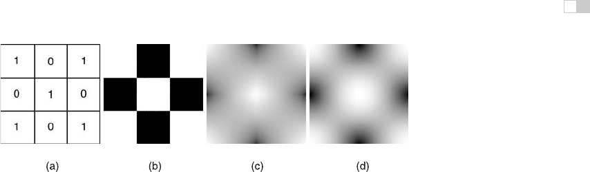
Figure 11.3. (a) The image on the left has nine pixels that are all either black or white. The
three interpolation strategies are (b) nearest-neighbor, (c) bilinear, and (d) hermite.
where
u
=3(u
)
2
− 2(u
)
3
,
v
=3(v
)
2
− 2(v
)
3
,
which results in Figure 11.3 (d).
In 3D, we have a 3D array of values. All of the ideas from 2D extend naturally.
As an example, let’s assume that we will do trilinear interpolation between val-
ues. First, we compute the texture coordinates (u
,v
,w
) and the lower indices
(i, j, k) of the array element to be interpolated:
c(u, v, w)=(1− u
)(1 − v
)(1 − w
)c
ijk
+ u
(1 − v
)(1 − w
)c
(i+1)jk
+(1−u
)v
(1 − w
)c
i(j+1)k
+(1−u
)(1 − v
)w
c
ij(k+1)
+ u
v
(1 − w
)c
(i+1)(j+1)k
+ u
(1 − v
)w
c
(i+1)j(k+1)
+(1−u
)v
w
c
i(j+1)(k+1)
+ u
v
w
c
(i+1)(j+1)(k+1)
,
(11.2)
where
u
= n
x
u −n
x
u,
v
= n
y
v −n
y
v,
w
= n
z
w −n
z
w.
(11.3)
11.1.3 Solid Noise
Although regular textures such as stripes are often useful, we would like to be able
to make “mottled” textures such as we see on birds’ eggs. This is usually done
..................Content has been hidden....................
You can't read the all page of ebook, please click here login for view all page.