

i
i
i
i
i
i
i
i
13
More Ray Tracing
A ray tracer is a great substrate on which to build all kinds of advanced rendering
effects. Many effects that take significant work to fit into the object-order ras-
terization framework, including basics like the shadows and reflections already
presented in Chapter 4, are simple and elegant in a ray tracer. In this chapter we
discuss some fancier techniques that can be used to ray-trace a wider variety of
scenes and to include a wider variety of effects. Some extensions allow more gen-
eral geometry: instancing and constructive solid geometry (CSG) are two ways
to make models more complex with minimal complexity added to the program.
Other extensions add to the range of materials we can handle: refraction through
transparent materials, like glass and water, and glossy reflections on a variety of
surfaces are essential for realism in many scenes.
This chapter also discusses the general framework of distribution ray trac-
ing (Cook et al., 1984), a powerful extension to the basic ray-tracing idea in which
multiple random rays are sent through each pixel in an image to produce images
with smooth edges and to simply and elegantly (if slowly) produce a wide range
of effects from soft shadows to camera depth-of-field.
If you start with a brute-
force ray intersection loop,
you’ll have ample time to
implement an acceleration
structure while you wait for
images to render.
The price of the elegance of ray tracing is exacted in terms of computer time:
most of these extensions will trace a very large number of rays for any non-trivial
scene. Because of this, it’s crucial to use the methods described in Chapter 12 to
accelerate the tracing of rays.
303
i
i
i
i
i
i
i
i
304 13. More Ray Tracing
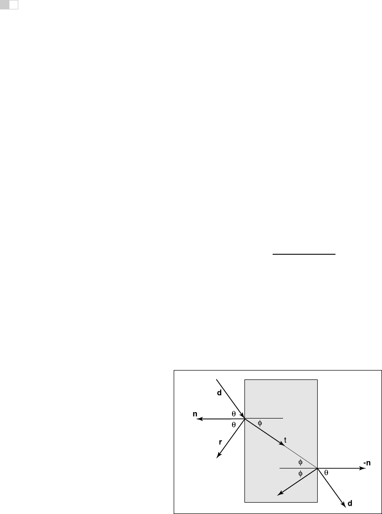
13.1 Transparency and Refraction
In Chapter 4 we discussed the use of recursive ray tracing to compute specular,
or mirror, reflection from surfaces. Another type of specular object is a dielec-
tric—a transparent material that refracts light. Diamonds, glass, water, and air are
dielectrics. Dielectrics also filter light; some glass filters out more red and blue
light than green light, so the glass takes on a green tint. When a ray travels from
a medium with refractive index n into one with a refractive index n
t
, some of the
light is transmitted, and it bends. This is shown for n
t
>nin Figure 13.1. Snell’s
law tells us that
n sin θ = n
t
sin φ.
Computing the sine of an angle between two vectors is usually not as convenient
Example values of
n
:
air: 1.00;
water: 1.33–1.34;
window glass: 1.51;
optical glass: 1.49–1.92;
diamond: 2.42.
as computing the cosine, which is a simple dot product for the unit vectors such
as we have here. Using the trigonometric identity sin
2
θ +cos
2
θ =1, we can
derive a refraction relationship for cosines:
cos
2
φ =1−
n
2
1 − cos
2
θ
n
2
t
.
Note that if n and n
t
are reversed, then so are θ and φ as shown on the right of
Figure 13.1.
To convert sin φ and cos φ into a 3D vector, we can set up a 2D orthonormal
basis in the plane of the surface normal, n, and the ray direction, d.
From Figure 13.2, we can see that n and b form an orthonormal basis for the
plane of refraction. By definition, we can describe the direction of the transformed
Figure 13.1. Snell’s Law describes how the angle φ depends on the angle θ and the
refractive indices of the object and the surrounding medium.

i
i
i
i
i
i
i
i
13.1. Transparency and Refraction 305
ray, t, in terms of this basis:
t =sinφb − cos φn.
Since we can describe d in the same basis, and d is known, we can solve for b:
d =sinθb − cos θn,
b =
d + n cos θ
sin θ
.
This means that we can solve for t with known variables:
Figure 13.2. The vectors
n and b form a 2D orthonor-
mal basis that is parallel to
the transmission vector t.
t =
n (d + n cos θ))
n
t
− n cos φ
=
n (d − n(d · n))
n
t
− n
"
1 −
n
2
(1 − (d ·n)
2
)
n
2
t
.
Note that this equation works regardless of which of n and n
t
is larger. An im-
mediate question is, “What should you do if the number under the square root is
negative?” In this case, there is no refracted ray and all of the energy is reflected.
This is known as total internal reflection, and it is responsible for much of the
rich appearance of glass objects.
The reflectivity of a dielectric varies with the incident angle according to the
Fresnel equations. A nice way to implement something close to the Fresnel equa-
tions is to use the Schlick approximation (Schlick, 1994a),
R(θ)=R
0
+(1− R
0
)(1−cos θ)
5
,
where R
0
is the reflectance at normal incidence:
R
0
=
n
t
− 1
n
t
+1
2
.
Note that the cos θ terms above are always for the angle in air (the larger of the
internal and external angles relative to the normal).
For homogeneous impurities, as is found in typical colored glass, a light-
carrying ray’s intensity will be attenuated according to Beer’s Law.Astheray
travels through the medium it loses intensity according to dI = −CI dx,where
dx is distance. Thus, dI/dx = −CI. We can solve this equation and get the
exponential I = k exp(−Cx)+k
. The degree of attenuation is described by
the RGB attenuation constant a, which is the amount of attenuation after one
unit of distance. Putting in boundary conditions, we know that I(0) = I
0
,and
i
i
i
i
i
i
i
i
306 13. More Ray Tracing
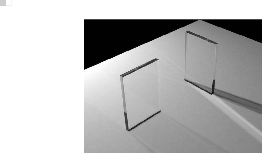
Figure 13.3. The color of the glass is affected by total internal reflection and Beer’s Law.
The amount of light transmitted and reflected is determined by the Fresnel equations. The
complex lighting on the ground plane was computed using particle tracing as described in
Chapter 24. (See also Plate IV.)
I(1) = aI(0). The former implies I(x)=I
0
exp(−Cx). The latter implies
I
0
a = I
0
exp(−C),so−C =ln(a). Thus, the final formula is
I(s)=I(0)e
−ln(a)s
,
where I(s) is the intensity of the beam at distance s from the interface. In practice,
we reverse-engineer a by eye, because such data is rarely easy to find. The effect
of Beer’s Law can be seen in Figure 13.3, where the glass takes on a green tint.
To add transparent materials to our code, we need a way to determine when
a ray is going “into” an object. The simplest way to do this is to assume that all
objects are embeddedin air with refractiveindex very close to 1.0, and that surface
normals point “out” (toward the air). The code segment for rays and dielectrics
with these assumptions is:
if (p is on a dielectric) then
r =reflect(d, n )
if (d · n < 0) then
refract(d, n,n,t)
c = −d · n
k
r
= k
g
= k
b
=1

i
i
i
i
i
i
i
i
13.2. Instancing 307
else
k
r
=exp(−a
r
t)
k
g
=exp(−a
g
t)
k
b
=exp(−a
b
t)
if refract(d, −n, 1/n, t) then
c = t · n
else
return k ∗ color(p + tr)
R
0
=(n − 1)
2
/(n +1)
2
R = R
0
+(1− R
0
)(1 − c)
5
return k(R color(p + tr) + (1 −R) color(p + tt))
The code above assumes that the natural log has been folded into the constants
(a
r
,a
g
,a
b
).Therefract function returns false if there is total internal re-
flection, and otherwise it fills in the last argument of the argument
list.
13.2 Instancing
An elegant property of ray tracing is that it allows very natural instancing.The
basic idea of instancing is to distort all points on an object by a transformation
matrix before the object is displayed. For example, if we transform the unit circle
(in 2D) by a scale factor (2, 1) in x and y, respectively, then rotate it by 45
◦
,and
move one unit in the x-direction, the result is an ellipse with an eccentricity of
2 and a long axis along the (x = −y)-direction centered at (0, 1) (Figure 13.4).
The key thing that makes that entity an “instance” is that we store the circle and
the composite transform matrix. Thus, the explicit construction of the ellipse is
left as a future operation at render time.
Figure 13.4. An instance
of a circle with a series of
three transforms is an el-
lipse.
The advantage of instancing in ray tracing is that we can choose the space in
which to do intersection. If the base object is composed of a set of points, one of
which is p, then the transformed object is composed of that set of points trans-
formed by matrix M, where the example point is transformed to Mp.Ifwehave
araya + tb that we want to intersect with the transformed object, we can instead
intersect an inverse-transformed ray with the untransformed object (Figure 13.5).
There are two potential advantages to computing in the untransformed space (i.e.,
the right-hand side of Figure 13.5):
1. the untransformed object may have a simpler intersection routine, e.g., a
sphere versus an ellipsoid;
..................Content has been hidden....................
You can't read the all page of ebook, please click here login for view all page.