
2.4 PETRI NETS FOR STATE MACHINES*
The finite state machines described earlier are sequential machines: only one state can be active at a time. This makes it difficult to design an FSM that is required to control parallel processes. One approach is to divide the specification into a number of sequential machines, which are linked together to implement a parallel controller. However, this does not explicitly represent the concurrency, and so makes it difficult to detect synchronization errors such as deadlock (when two processes are waiting for each other). A more satisfactory method of representing the concurrency is to use a single parallel controller that can have several states active simultaneously. Such a parallel controller can be represented using a Petri net model. This gives a clear specification of the parallelism in the design. The specification can then be analyzed for correctness, and used as a basis for the implementation.
2.4.1 Basic Concepts
A Petri net is a directed graph comprising nodes of two kinds—places and transitions—and directed arcs that connect places to transitions and vice versa. Places are commonly represented by circles and transitions by bars. A place can contain a token, which is depicted as a black dot. A marking of a Petri net is a mapping of a set of tokens to places in the net. The behavior of the system represented by the Petri net is defined by the movement of tokens. A simple Petri net is shown in Figure 2–10.
In the general case, arcs can be labeled with integer numbers that describe how many tokens are carried through a particular arc when the tokens move around the net. Petri nets involving arcs that are able to carry only one token at a time are called ordinary Petri nets. The following sections are restricted to the consideration of ordinary Petri nets.
Tokens can proceed through a Petri net according to a certain rule called a transition firing rule. To define this rule some other definitions have to be introduced.
The input places of a transition are the places that are connected to the transition by arcs leading from those places to the transition. Similarly, the output places of a transition are the places connected to the transition by arcs leading from the transition to those places. A transition is enabled if each of its input places contains at least one token. If a transition is enabled, it may fire. A firing of a transition removes a token from each of its input places and adds a token to each of its output places. Figure 2–11 shows a Petri net before and after the firing of transition T2.
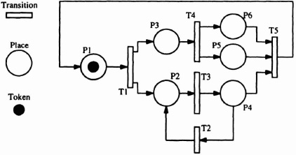
Figure 2–10. Simple Petri net.

Figure 2–11. Petri net before (a) and after (b) transition T2 fires.
All enabled transitions fire asynchronously, subject to the rule presented previously with the restriction that tokens are indivisible. In Figure 2–11b both transition T4 and transition T5 are enabled, but only one of them can fire since they share an input place holding a token. Firing either of them disables the other. Such a situation is called a conflict. When a conflict arises in a net, the choice of which transition to fire is arbitrary. If a system that is represented by a Petri net is to be deterministic, all conflicts must be removed from the net.
2.4.2 Basic Properties
A Petri net representation of a system can be used as an input for analyzing behavioral properties of the system [Murata89]. Two properties are essential to ensure that a system described by a Petri net is to work correctly. The properties are liveness and boundedness (or safeness). Both liveness and boundedness are strictly connected not only with a structure of a net but also with an initial marking. A Petri net with a marking is called a marked Petri net. When describing the properties just mentioned, marked Petri nets will be considered.

Figure 2–12. Nonlive Petri net.
A Petri net is said to be live if for any marking reached from the initial marking it is possible to fire any transition of the net by progressing through a firing sequence. If a Petri net representation of a system is live, it means that there is no deadlock in the system. The Petri nets shown in Figures 2–10 and 2–11 are live. Figure 2–12 gives an example of a nonlive Petri net.
It is nonlive because when P1 and P4 have tokens and T2 fires no further firing is possible. The net would be live if it could be guaranteed that whenever the marking is P1, P4 only T1 could fire.
A marking M is said to be reachable in a Petri set N with the initial marking M0 if there exists a firing sequence that transforms M0 to M. A Petri net is said to be bounded (or k-bounded) if the number of tokens in each place does not exceed a finite number (a finite number k) for any reachable marking [Murata89]. Safeness is a special case of boundedness. A Petri net is said to be safe if the number of tokens in each place never exceeds one. Figure 2–13 shows Petri nets that are safe, 2-bounded, and unbounded, respectively.
Some bounded although nonsafe, or even unbounded Petri nets can be considered as bounded ones when some restrictions are imposed on the transition firing rule.
2.4.3 Extended Petri Nets for Parallel Controllers
To describe digital controllers using the Petri net model, each place is used to represent a local state in the controller. The marking, or global state, is obtained by concatenating these local states and mapping them onto the controller’s state register. Transitions map onto the combinatorial logic block. Resetting the controller returns the Petri net to its initial marking. The model is extended in the following three ways:

Figure 2–13. Safe (a), 2-bounded (b), and unbounded (c) Petri nets [Murata89].
- Transition enabling is modified by optionally attaching a predicate to each transition, where each predicate is a Boolean function of the controller’s input signals. A transition is now enabled if all of its input places are marked and its predicate, if present, is asserted.
- The Petri net is synchronously clocked so that its marking is only updated at the start of each clock cycle. Transitions fire when the clock is active provided the inputs and other conditions enable the transitions to fire. This will then create a new marking in the net.
- The controller’s output signals are attached to selected nodes in the Petri net, and are asserted whenever any of their associated places are marked (for Moore outputs) or transitions are enabled (for Mealy outputs).
This model of the Petri net provides all the features needed to allow the representation of digital controllers. However, for complex designs the net can be simplified by using enabling or inhibiting arcs. These are additional predicates on a transition that originate from a place somewhere else in the net. When a transition has an enabling arc attached to it, it can only fire when the place connected to the enabling arc contains a token. The token does not move as a result of the transition firing. When a transition has an inhibiting arc attached to it, then it can only fire when there is no token present on the place connected to the inhibiting arc. An illustration of the use of enabling and inhibiting arcs is given in the frame-store example discussed in Chapter 5.
Adding enabling or inhibiting arcs makes the net less easy to test, since it can introduce deadlocks not detectable by the normal liveness tests. Transformation techniques exist to tum a net with enabling/inhibiting arcs into a near-equivalent standard Petri net form, sufficiently good to allow liveness tests to be carried out.
2.4.4 Simple Example—A Traffic Light Controller
A traffic light controller* can be described using the Petri net notation and more naturally allows the description of the controller function. Consider a crossroads with lights N-S and E-W. The light colors are red, amber, and green. The N-S flow and the E-W flow are controlled by lights with the same pattern. Thus the normal sequence would be:
![]()
The sequence is described by the central pattern in the PN of Figure 2–14. The lights are defined by the places P1 to P8 The transitions T1 to T8 would be enabled by timers designed to give the required interval for each light phase. While this core sequence can be described by an ordinary FSM technique, the power of the PN becomes apparent if a more complex specification has to be realized. For example, the lights can be allowed to remain green until traffic is detected on the other road. The loops P9: T9: P10 and P11: T10: P12 deal with this situation. Places T9 and T10 are enabled by a sensor detecting a vehicle in the east–west and north–south roads, respectively. Only when a token reaches P10 and P12 will the light sequence continue, provided that the time-outs for T5 and T1 have finished.
An even more exotic arrangement could count the vehicles, perhaps to allow a longer time period when a high flow rate is detected. The two loops P13: T11 and P16: T12 count vehicles: T11 and T12 are enabled when the sensor detects a vehicle, and P13 and P16 increment a counter. The counting process is stopped when the corresponding road gets a green light, that is, T8 or T4 fires. This causes P14 and P17 to acquire a token, which allows T13 and T14 respectively, to fire, removing the token from P13 and P16 in the counting loop. The action places tokens in P15 and P18, allowing the counting sequence to be reenabled for next time.

Figure 2–14. Traffic light controller.
The initial marking is important and not obvious. Clearly it is desirable to start on RNRE, that is P3 or (P7). (From here on, the items in parentheses are an alternative marking.) The other markings must ensure that the counting nets are live. By inspection, it is clear that a token needs to be available to allow T14 (T13) to fire when P17 (P14) receives a token from T4 (T8), so a token in P16 (P13) is necessary.
Also, if the E-W (N-S) counting sequence is to be activated, then there need to be tokens in P9 (P11) and P15 (P18). (There may be other initial markings that are perhaps simpler, but they will not ensure a safe starting point for the traffic on the junction: for example, a more logical initial marking would be P1: P12: P15.)
2.4.5 Implementation of Petri Net Description
The implementation of the Petri net can take one of many forms. There are three currently developed methods that yield good results. One technique is to identify partitions of the net, which become linked finite state machines. Each state machine may then be implemented using the methods described earlier. Another approach is to identify sequential portions of the machine as macro places or macro transitions, thereby reducing the net to its parallel constituents only. These parallel states are then allocated unique state variables. The rest of the places are coded using the states of the macroplace and sufficient new state variables to encode the places uniquely. This approach results in an efficiently implemented design using a small number of flip-flops.
The most straightforward approach, however, is to assign one flip-flop to every place in the net. This is analogous to the one-hot encoding for FSMs described earlier in the chapter. For a design to be implemented in an FPGA with plenty of flip-flops, such as a logic cell array (LCA), this is an acceptable approach [Schlag91]. All flip-flops are cleared at power-up. The ones with an initial marking have inputs and outputs inverted, so their outputs are asserted at the outset. The basic features are (1) feedback around each flip-flop for it to retain its token, and (2) a previous synchronous reset fedback to all preceding flip-flops to clear tokens as they move across a transition.
The example in Figure 2–15 shows a small part of a net together with its implementation. The net consists of initially marked place P1, normal place P2, and transitions T1 and T2. Input A to T1 and input B to T2 are from other places in the net.
The flip-flop for place P2 can be seen to be set, on “DC,” when the output from T2 is high. It remains set as the bit is recirculated, until the reset signal from the subsequent place is asserted (by which time the output from T2 will be low again). Place P1 is similar, but with the flip-flop input and output inverted to implement the initial marking. Since transitions fire when all input conditions are satisfied, they are simply AND gates when there is more than one input, as for T2, or nothing, as for T1.
This form of implementation is very straightforward and can be easily automated. Furthermore the simplicity of the circuitry is well-suited to small combinational blocks of logic, such as the configurable logic blocks (CLBs) inside an LCA. In most cases, a flip-flop and the preceding Boolean expression fit into one CLB. An implementation with more economical flip-flop usage would result in many more high fan-in logic functions, which would have to be split between multiple CLBs and could potentially slow the machine down.

Figure 2–15. Implementation of a Petri net fragment.
A small amount of minimization can be done where a small net of two states exists. These can be readily implemented by a single flip-flop rather than two.