6.5    SELF-TIMED GENETIC STRING DISTANCE EVALUATION

6.5.1    String Comparison

The string comparison problem is to find the minimal distance between two strings from a user-defined alphabet set, where the distance between two strings is defined as the cost of transforming one string into the other. Any string can be transformed into another with the aid of the operations insert, delete, and substitute. Distance is considered as the weighted sum of such operations. For example, one way to turn ‘ATGC’ into ‘AATG’, would start by substituting the second letter ‘T’ in ‘ATGC’ with ‘A’, substituting the letter ‘G’ in ‘ATGC’ with ‘T’, and substituting the fourth letter ‘C’ with ‘G’. Alternatively, we could insert an ‘A’ before ‘ATGC’, and delete the fourth letter, ‘C’, in ‘ATGC’. If we define the cost of both insertion and deletion operations as ‘1’, and a substitution operation as ‘2’, then the distance between ‘AATG’ and ‘ATGC’ is ‘6’ using the first method, and ‘2’ with the second. In the absence of any better alternative, the minimal distance between ‘AATG’ and ‘ATGC’ is ‘2’.

String comparison is a common and important operation in almost all information retrieval systems, such as text retrieval, dictionary searching, and biomorphic database retrieval. It is regarded as one of the Grand Challenge computing problems of this decade.

6.5.2    Genetic Sequence Comparison

The genetic sequence comparison problem is a special case of the string comparison problem applied in the field of molecular biology. Spectacular advances in medicine have come from the decoding of genetic material and the comparison of chains from different organisms. While there are only four characters in the genetic “alphabet,” chains may be hundreds of thousands of characters in length. There is a growing data base of decoded genetic material, which is regularly searched for close matches for a newly determined chain. A chain of DNA consists of the four bases, adenine, cytosine, guanine, and thymine, which are abbreviated A, C, G, and T, and so the alphabet set for Genetic Sequence Comparison problem is (A, C, G, T). Given a chain of DNA as the source string, we need to compare it with any chain from a data base of known DNA and find the DNA structures with the minimal distances from the source DNA chain.

6.5.3    Dynamic Programming Algorithm

Given two genetic sequences, we want to find the minimal distance between them. Fortunately, this problem has an optimal substructure property, which allows us to use dynamic programming techniques. This property appears to have been discovered by Levenshtein [Kohon87]. Let X = (x₁, x₂,x₃,...,x_m) and Y = (y₁,y₂,y₃,...,y_n) be two input strings. Let d_i,j, be a minimal distance between (x₁,x₂,...,x_i) and (y₁,y₂,y₃,...,y_j). Then,

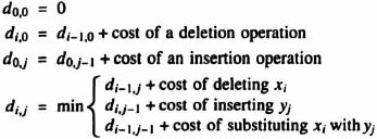
(If x₁ = y_j, then the cost of substituting x_i with y_j is 0.)

If we store the distance values in a matrix, the optimal substructure determines that each value d_i,j in the matrix depends only on the values of the antidiagonal lines above and to the left. A dynamic programming algorithm based on the preceding optimal substructure property is then used to solve the string comparison problem. As an example, here is the distance matrix by applying the dynamic programming algorithm to the comparison of AATG with ATGC:

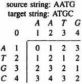
The matrix contains the distances for substring comparisons as well as the final distance in the lowest right-hand element. In consequence, what appears to be a quadratic problem can in fact be solved with a linear array of processing elements.

6.5.4    Implementation Considerations

Many different implementations of this well-known dynamic programming algorithm have been developed. Lipton [Lipton85] presented a linear systolic array implementation using an nMOS prototype, later to be known as Princeton Nucleic Acid Comparator (P-NAC), to be used in searching genetic data bases for DNA strands. The source and the target strings are shifted into an array of processing elements (PEs) simultaneously from the left and the right, respectively. Each character is separated by a null element so that simultaneous left and right shifts may be performed without missing any character comparisons. This is referred to as the bidirectional algorithm. When two nonnull characters enter a PE from opposite directions, a comparison is performed. A clock is used to control the data flow, and all PEs can work in parallel. To compare two strings of length n in one pass requires 2n PEs. Subsequently, the algorithm was used with the SPLASH 1 and SPLASH 2 architectures, which consist of regular arrays of Xilinx 3000 and 4000 series FPGA chips, along with considerable amounts of RAM. These implementations gave higher performance as well as opportunities for exploring variations in the basic algorithm. Hoang [Hoang93] reported a SPLASH 2 implementation for the algorithm, which could search a data base at a rate of 12 million characters per second. Hoang also developed an interesting variant known as the unidirectional algorithm. This requires only half the number of PEs, that is, n. The source string is loaded at the outset by storing it in the array, starting from the leftmost PE. It allows multiple string comparisons by streaming target strings through the array one after another, with a control character separating each string.

It is clear that applying the algorithm to problems of serious interest in molecular biology will require literally hundreds of thousands of PEs, and it will be difficult to synchronize their operation with a conventional clocking scheme. Following earlier work with self-timed micropipelines, we decided to implement a small-scale version of the unidirectional algorithm on an array of Algotronix CAL1024 FPGA chips. The CAL architecture has a number of attractive properties for this application:

1. The fine-grain architecture is economic for self-timed primitives.
2. The chip I/O pad arrangements allow vertical and horizontal cascading without limit.
3. The array can be dynamically reconfigured in an incremental manner.

Some of these general features are illustrated in Figure 6–27, as implemented on an Algotronix CHS2×4 board which fits into a standard IBM PC or clone. Each chip can hold two PEs. There is a start-up stage where we load the source string and initialize the pipe of PEs. Since the organization is self-timed, there are no synchronization issues, even allowing for the delay in crossing chip boundaries, and the design runs at its maximum speed as well as being simple.

Figure 6–27. CAL board.

6.5.5    Performance Evaluation

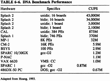
Hoang [Hoang93] used the number of cells (entries in the distance matrix) updated per second (CUPS) to measure the performance of an implementation, and we have simply added an entry to the published table (see Table 6-6). The generated delay for each PE in our implementation is 440 ns. If a pipe has N PEs, then the pipeline is capable of 2.273 × N MCUPS with the Algotronix CAL. Note that the CAL implementation assumes 384 PEs.

6.5.6    The Self-timed Implementation*

The Algorithm   Imagine that in the pipeline shown later in this section, the target string T_j−2, T_j−1, T_j, T_j+1 is flowing through the array of processor stages. In the stages, source values S_i−1, S_i, S_i+1, S_i+2 are held, one per stage (see Figure 6–28).

Calculating the distance in stage i,d_i,j then becomes a matter of simply choosing the minimum from (d_{i−1, j}) + 1, (d_i,j−1) + 1, or P. If T_j is equal to S_i, P has a conditional value of (d_{i−1, j−1}) or (d_{i−1, j−})+2 otherwise. Once stage i + 1 accepts target value T_j, the distance value calculated in stage i is pushed onto a two-position stack. This allows memory of past d_i,j−n distances for use in future distance calculations.

Figure 6–28. Pipeline of processor elements.

Why Self-timed?   There are three potential advantages in making a self-timed implementation of an algorithm.

• Reduced power consumption
• Ease of design, which in this example, translates into infinite cascadability
• The ability for a circuit to run at its maximum speed, instead of assuming the worst-case speed, as for a synchronous alterative

Our implementation fully capitalizes on the first two advantages, but does not utilize the potential speed gain. In a clocked system, all stages experience a rising and falling of a clock signal. In self-timed pipelines like this one, one edge is used instead of two, and that single edge is only present in active stages. Idle stages experience no edge at all. The simplicity of design was the main motivation for this self-timed implementation. If it is attractive to the user of this genome distance calculator to have 25,000 chips placed end to end, then that user may do just that with no consideration of clock skew or synchronization problems. In order to make the components of the PE as simple and straightforward as possible, they are not internally self-timed. The worst-case time of the PE was accurately calculated (440 ns), and an equal delay is generated using propagation through buffers of a forward request signal. This design decision robs the design of its potential speed within chip, but still allows for delay variation at chip boundaries.

The Implementation   The pipe is made of type-A elements and type B elements in an alternating fashion (see Figure 6–29). There is a type B element between each two type A elements, and therefore the first and last elements are type A elements. The type A elements are stacks with adders, and the type B elements find the minimum of three numbers.

The recursive part of the algorithm is implemented as follows. Suppose a type B element is in stage i with target character T_j passing the stage. When the type B element determines the minimum distance, corresponding to d_{i, j}, it takes its first input from the top of the stack of its left-hand type A element, with one added to it, that is, d_{i−1, j} + 1. It takes another input from the top of the stack in its right-hand type A element, again with one added, that is, d_{i, j −1} + 1. The third input comes from the bottom stack of its left type A element, which holds the value d_{i−1, j −1}. Now the target character is compared with the source character. If they differ, 2 is added to the value, stored in the bottom stack of its left type A element. Otherwise the characters are the same, and the distance is passed onto the type B element unchanged. This element passes on the result to the next stage by placing it on the top of the stack in its right-hand type A element. From the top of the stack, 1 is added to the value, as stated in the algorithm.

Figure 6–29. Type A and type B stages.

Figure 6–30 shows a complete processing element as implemented in Algotronix CAL, with its subunits unexpanded, while Figure 6–31 is fully expanded. Figure 6–32 shows the minimum unit.

Control   The pipeline is controlled with a standard micropipeline handshaking protocol as described in Sutherland’s 1989 Turing award paper, “Micropipelines” [Suther89], There is a fixed delay of 440 ns placed between the Muller-C output and the uninverted input of the next stage (see Figure 6–33).

There is one event that occurs between the control structure and the stacks that lie in the type A stages that is not standard protocol for a micropipeline. When the Muller-C elements are being forcefully cleared by a global clear signal, the stacks do not hold any events caused by this operation. Therefore, the pipeline can be filled with values and the stacks can be set according to the calculations that take place in the pipeline. Then the pipeline can suddenly be emptied, but retain the data values that were formed in the filling process. This is needed in the loading process.

Loading Source Values   Originally, the pipe is empty. The source values are entered into the pipe from the left side with a standard request-acknowledge protocol. During this loading process, the initial distance of each source character is loaded in each stage.

Figure 6–30. CAL layout of a single stage of the pipeline (hierarchical).

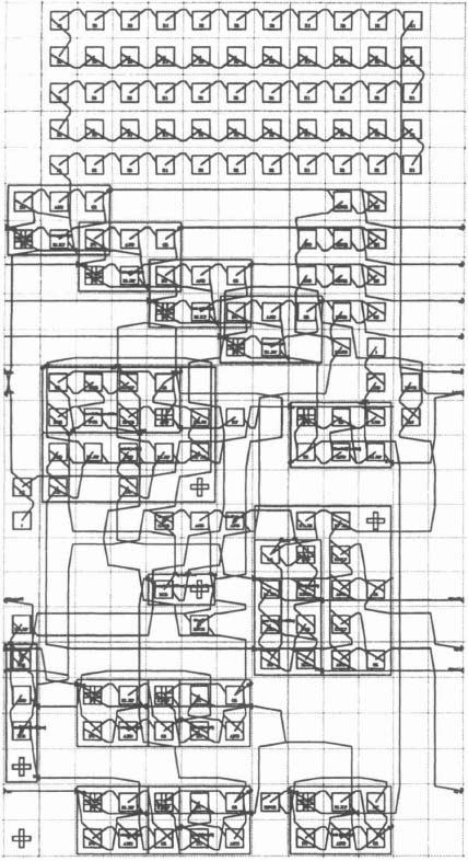
Figure 6–31. CAL layout of a single stage of the pipeline (fully expanded).

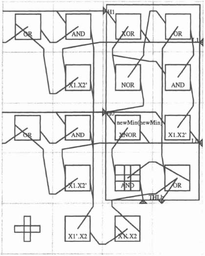
Figure 6–32. CAL block for minimum determination.

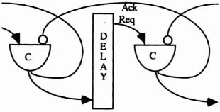
Figure 6–33. Self-timed signaling.

The Algotronix CAL architecture has two global lines, G1 and G2. In order to signal the pipeline that loading is in progress, G1 is set to 1 and held high throughout loading. While G1 is high, the MIN calculator in the type B stage shuts down, and simply passes the value that enters from the left side of the B cell. The top of each stack adds one to the distance value that it receives from the left. The user must set the proper initial distance value to be entered into the pipeline from the left stage. The formula for the initial distance is given later in this section.

If the source string has length s, and the pipe has n stages, then the number of empty stages is e = n − s. It is important that the leftmost source value stored in the pipeline has the distance value 1. In order to guarantee this, an initial distance must be entered in the left-hand side of the pipe that has a modulo 4 sum of 0 in the last empty stage. The formula d_i = (4 − (e mod 4)) mod 4 gives that distance. This input distance is the same for all source characters. The entire source string may then be entered using the request-acknowledge protocol (see Figure 6–34). Note that the modulo 4 scheme allows an arbitrary number of PEs to be cascaded, that is, it is totally scalable.

Once all source values are loaded, G1 is lowered, then G2 is lowered and raised again in order to forcefully clear the FIFO control lines. The data values of source and distance are maintained in the stages during this clear procedure.

Empty Stages   The pipeline may be longer than the source string. If this is the case, it is important for a stage to know that it is empty. Using a micropipeline, it is obvious that a stage is empty whenever Req is equal in value to Ack. This can be seen in Figure 6–33.

The global signal G1 is lowered at the end of the loading of the source value. When it is lowered, the source characters are latched in the stages. The empty signal for each stage is also latched, so any stage that is empty at the end of the loading process, is given a permanent Empty signal. These stages act as nonprocessing FIFO stages in the distance calculation.

Conclusion   The self-timed organization is attractive for problems of substantial size, and adapts to variations between individual chips as well as chip-chip boundary delays. It is scalable, and adaptable to alphabets of different size. Thus it could be adapted to the protein sequence problem which requires a set of about 15 distinct characters. The CAL1024 chips used in this experiment were implemented in 1.5-μ CMOS technology, and would be faster as well as denser with current submicron fabrication technology. While any large-scale implementation would justify the design and fabrication of a full-custom chip, with both higher density and speed, FPGAs allow rapid prototyping of a detailed design as well as experiments, such as different weight factors. Distance evaluation is only one aspect of the overall requirement, and further work is needed in the recognition of multiple subsequences and other structural features in string comparison.

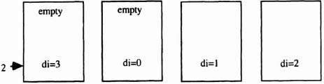
Figure 6–34. Initial loading of pipeline distances.