
6.6 CELLULAR AUTOMATON
Recently, much attention has been focused on cellular automata simulations of physical problems: [Wolfram86] contains a collection of important cellular automata papers, and [Toffoli87] provides a much more approachable introduction to the topic based on one particular cellular computer, the CAM-6.
The goal of these models is to set up a “universe,” based on a particular cellular automaton rule that mimics physical reality in some way, and observe its evolution. This is to be contrasted with the more traditional approach in [Prest84], where automata are used as data-processing devices to produce desired transformations in image processing. Of particular interest are the cellular automata models for fluid flow simulation: currently, a large fraction of the world’s supercomputer time is consumed by this type of problem, and cellular automata models promise cheaper and more powerful computers for this application. Although there was initially a degree of skepticism about cellular automata models in the physics community, much work has been done in the last few years in validating the cellular models, and they have gained wide acceptance. Validation has been done both against experimental results and by showing mathematically that the cellular models approach known differential equations (e.g., the Navier-Stokes equation) for particular “regions” of interest.
In this section, we outline the design of a CAL-based machine for solving such problems. This work was originally presented in [Kean89].
6.6.1 The Model
The most commonly used cellular automaton rule for fluid flow simulation is called hexagonal lattice gas and simply specifies what happens when molecules collide on a hexagonal grid. All molecules are assumed to have the same mass and velocity: the density of the grid (i.e., the proportion of lattice sites that are populated at the start of the simulation) is proportional to the fluid’s Reynold’s number. An example rule is shown in Figure 6–35. In the “before” step all the arrows face toward the current site and in the “after” step all the arrows face away: thus the situations can be coded as six-bit numbers representing the presence or absence of a particle traveling in a particular direction. Note that to model real fluids properly the rules must obey certain physical properties (e.g., conservation of momentum) and are symmetrical with respect to rotation and reflection.
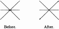
Figure 6–35. Example lattice gas collision rule.
To obtain interesting results we usually wish to place some object within the fluid. At those sites on the edge of the object a different set of rules will be used, for example, particles reflect back with angle of reflection equal to angle of incidence. It is inefficient to reconfigure the update unit when these sites are being computed, so the normal technique is to add an extra bit plane that contains 1s along the outline of the obstacles. We then use an automaton rule with 7 inputs and 6 outputs (since the obstacles do not move) specified as the normal 6-bit rule when the seventh plane is 0 and the reflection rule when it is 1.
The rule in Figure 6–35 does not use a true hexagonal grid, but has approximated the hexagon on a rectangular grid using 45° diagonals: this is an acceptable transformation in most cases and is necessary to match the structure of the RAM memory that will hold the model points. In some cases a more accurate approximation will be required; this approximation involves a slight increase in complexity and some unused store in the RAM.
Another point of interest is that the “after” stage in our example is not the only one that conserves momentum—particles could also leave on the other two diagonals. Rules that make random choices between different possibilities are also of interest and can offer increased accuracy. While it is inefficient to add randomization at each individual node update, other techniques, for example, using one possibility on “odd” lattice sites and the other on “even,” or using one possibility on “odd” update cycles, can be used and are reasonably effective.
Although the basic computation is very simple, to get good results it must be repeated on an extremely large grid of points (2048 × 2048 is not uncommon) and perhaps 10,000 iterations must be run between samples. One such cycle would involve about 42 × 109 node updates. The need for parallel processing is obvious. After enough cycles have been run, the model is divided up into larger sectors with about 64 sites per sector. The average direction of the molecules within each sector is converted into an arrow, whose length represents the number of particles heading in the most common direction and a diagram such as Figure 6–36 is produced, clearly showing the structure of the flow. The site data can also be used to calculate numbers of interest, such as forces on obstacles and pressures, after calibrating the model appropriately.

Figure 6–36. Example of output from lattice gas model.
6.6.2 Architecture
There are several methods of organizing the update computation.
- One Processor per Site. This is the obvious method, using a hexagonal grid of processors and communication between them to deal with particle movement, but it is not practical for real models with as many as 4 million sites.
- Single Phase. In this implementation the calculation consists of both particle movement and site computation. Enough memory is provided within the computation unit to store the values of all sites adjacent to those whose new values are now being computed. Each site takes the inputs for its computation from the memory corresponding to adjacent sites (converting arrows leaving the adjacent site in the “after” phase of the rule to arrows entering this site for the “before” phase). This method is very easy to use when only a single update processor is available, but the routing becomes complicated when several updates take place in parallel (because of the need to store “before” values for a given site after its new value is computed to allow adjacent nodes to perform their update).
- Two Phase. In this approach [Clouq87] the memory subsystem is treated as several bit planes, and the values in the planes at a particular address correspond to the “before” data for the corresponding site. The computation unit performs the update and writes back the new “after” value as shown in Figure 6–37. After all sites have been updated, the memory subsystem manipulates bit-plane address offsets to perform a separate “movement” phase in which the bit planes are “realigned” so that in the next computation sweep, cells again have “before” values. For example, to move a bit plane “up,” one would add an offset of the number of pixels in a row. This assumes that memory addresses ‘wrap around’ at the edge of the bit plane. Wraparound is actually very desirable in a cellular automaton system, since otherwise the fact that edge sites have no neighbors in one direction can distort the results. This approach is very easy to implement, involves almost no performance penalty, and simplifies the design of the update unit. We will assume the two-phase approach in this design, although because the circuitry is reconfigurable, it could also implement the single-phase method.

Figure 6–37. Basic lattice gas simulator architecture.
Performance Goals Before starting out on a design like this, it is important to consider the performance required. Supercomputer implementations of automata problems currently achieve 109 site updates per second, so we will take this as our goal and assume that we are working with 2048 × 2048 site lattices. Since 4M 7-bit words of memory are required for this size of model and 4096 × 4096 site models are already being suggested, we also require that the memory subsystem be implemented using cheap dynamic RAM.
Update Unit Implementation The first thing to consider is the best way to implement the site update computation with the CAL architecture. We note that the case where the “object” bit plane is 1 is very simple, since reflection simply involves a swapping operation on inputs. For use of a CAL with a read-only control store—a CAL-ROM—seems appropriate for the hexagonal-lattice-gas rules when no object is present. We can integrate the reflection unit with the CAL-ROM as shown in Figure 6–38. Note that for clarity the pipeline registers are not shown in this figure.
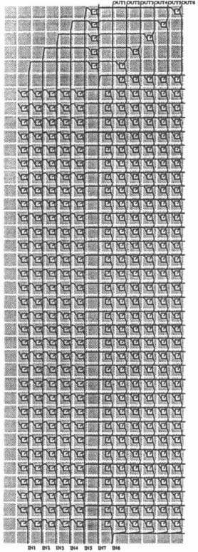
Figure 6–38. Layout of single update unit.
We have n = 6, m = 6, p = 32, so using the parameters for CAL256 delay given in section 6.3.3 and assuming 4 product terms per pipeline stage, the delay is 5 × 10 + 5 × 2.7 + 4 × 10 = 103.5 ns. There are eight pipeline stages in the ROM, plus one for the extra multiplexing. Use of dynamic memory suggests a pipeline tick of 120 ns to allow a memory access to occur and data be routed to the CAL in a single cycle. We will assume that 64 × 64 cell chips are being used: each CAL-ROM is 11 cells high and an extra line of cells is needed to route the seventh bit plane, giving a total height of 12 cells. This allows five units per chip. Assuming that the multiplexers use a fairly sparse layout 6 cells wide, we have a total width of 32 (product terms) + 6 (multiplexer) + 18 (pipeline registers) = 56 cells. We still have 4 spare rows and 10 spare columns of cells on each chip for any other circuitry we may want, for example, wiring channels to simplify off-chip routing. With 128 computation units (using 26 CAL chips) we can do 1.07 × 10⁹ updates per second.
Memory Subsystem In order to achieve the very high data rate (6 × 128 = 768 bits every 120 ns) required, a special purpose memory subsystem is necessary. We will consider the design of one bit “plane”; all the bit planes can be identical. Each bit plane must provide 4M bits of RAM and deliver 128 bits every 120 ns. If we choose memory chips that output 4 bit words, then we need to access 32 chips. We also have to simultaneously write back information from the CAL into the bit-plane memory. Given these considerations, a single 4M bit-plane memory could be built from two banks of 32 cheap 16K × 4 (64K) dynamic RAMs (Figure 6–39). Larger 4096 × 4096 site models are already being suggested, so a version of the system with 64K × 4 memories is also worth considering.
The addressing circuitry required is shown in Figure 6–40. Note that we need to decrement the address from which data are being read by the number of stages in the pipeline to get the write address. Each bit plane is assumed to receive the current “site” address from a global controller. Naturally, all this control circuitry would be implemented using CAL chips to provide maximum flexibility.
6.6.3 Comparison with Previous Systems
The configurable logic architecture differs from previous special-purpose cellular automaton machines by having many processors and using configurable ROMs rather than lookup tables for calculations. The main disadvantage of the lookup technique is that the size of the RAM required grows as 2n with the number of inputs n. RAM size and number of processors must also be fixed in advance—you do not get more processors when the rule is simple. Cellular automaton models with as many as 24 inputs have been suggested to increase the accuracy of the simulations. Naturally, if the rules were completely random functions of n variables, configurable logic could do no better than lookup tables: however, cellular automata rules for lattice gas equations are very regular (this follows from basic properties of the physical model, such as symmetry and conservation of momentum). We can see the advantages of the. configurable logic approach from the preceding example: if a RAM lookup table had been used, then the size of the RAM would be doubled by the seventh input bit. However, with the CAL implementation only a very small additional piece of logic is required. It is likely, therefore, that despite the number of inputs in the newer rules, an implementation using relatively few logic gates will be possible. The structure of this implementation will vary from rule to rule. In the lattice gas model of this example, rotation and reflection symmetry could be used to reduce the number of rules from 64 to 14 [Wayner88].

Figure 6–39. Architecture of single bit plane.
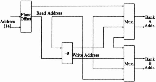
Figure 6–40. Memory addressing for one plane.
TABLE 6-7. Performance on Fluid Flow Simulations
| System | (Site Updates/Second) × 106 |
| Cray X/MP | 500 |
| Connection Machine | 1000 |
| Single Princeton Chip | 20 |
| Princeton system | 1000 |
| Single 64 × 64 CAL | 40 |
| CAL system | 1070 |
With a reasonable amount of hardware the configurable logic system can easily outperform any conventional computer on this problem: Table 6-7 compares the expected performance of the system with supercomputer implementations and custom chips. The first Princeton figure is a maximum per chip. There are 1500 chips in the present configuration. However, I/O considerations on the SUN-3 host limit the performance per chip to 2/3 million sites/second, giving an overall performance of 1000 million sites/second. This figure is disappointing for a custom chip and is a result of the method of organizing the computation to reduce I/O bandwidth and avoid the need for a special memory subsystem—75% of the Princeton chip area is taken up with a large shift register, and there are only two update units per chip. The Princeton chip uses 3-μm technology rather than the 1-μm technology needed for a 64 × 64 cell CAL. The Connection Machine and Princeton chip figures come from [Wayner88], and the figures for the Cray supercomputer are from [Shimom87]. The CAM-6 and RAP systems mentioned previously do not support enough lattice sites and have much lower performances because they have only one lookup table for site update calculation.
6.6.4 Conclusion
We can see that the CAL design is extremely cost effective, providing supercomputer performance from a system with fewer than 30 custom chips (even including control circuitry) and less memory than a low-end workstation. Even when the cost of a host computer to control and display the results of the simulations is included, the system is very attractive. The use of reconfigurable chips in the update and control units will allow this system to evolve as the models become more complex. Also, extra memory planes and larger update units are easily accommodated.