
i
i
i
i
i
i
i
i
23.6. Gradient-Domain Operators 607
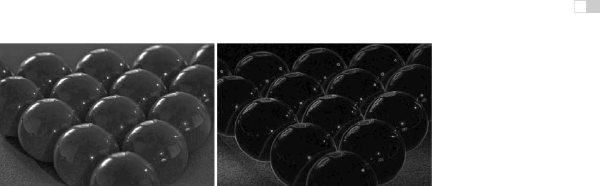
Figure 23.16. The image on the left (tonemapped using gradient-domain compression)
shows a scene with highlights. These highlights show up as large gradients on the right,
where the magnitude of the gradients is mapped to a grayscale (black is a gradient of 0,
white is the maximum gradient in the image).
23.6 Gradient-Domain Operators
The arguments made for the frequency-based operators in the preceding section
also hold for the gradient field. Assuming that no light sources are directly visible,
the reflectance component will be a constant function with sharp spikes in the
gradient field. Similarly, the illuminance component will cause small gradients
everywhere.
Humans are generally able to separate illuminance from reflectance in typical
scenes. The perception of surface reflectance after discounting the illuminant is
called lightness. To assess the lightness of an image depicting only diffuse sur-
faces, B. K. P. Horn was the first to separate reflectance and illuminance using a
gradient field (Horn, 1974). He used simple thresholding to remove all small gra-
dients and then integrated the image, which involves solving a Poisson equation
using the Full Multigrid Method (Press et al., 1992).
The result is similar to an edge-preserving smoothing filter. This is accord-
ing to expectation since Oppenheim’s frequency-based operator works under the
same assumptions of scene reflectivity and image formation. In particular, Horn’s
work was directly aimed at “mini-worlds of Mondrians,” which are simplified
versions of diffuse scenes which resemble the abstract paintings by the famous
Dutch painter Piet Mondrian.
Horn’s work cannot be employed directly as a tone reproduction operator,
since most high dynamic range images depict light sources. However, a relatively
small variation will turn this work into a suitable tone reproduction operator. If
light sources or specular surfaces are depicted in the image, then large gradients
will be associated with the edges of light sources and highlights. These cause the
image to have a high dynamic range. An example is shown in Figure 23.16, where
the highlights on the snooker balls cause sharp gradients.
i
i
i
i
i
i
i
i
608 23. Tone Reproduction
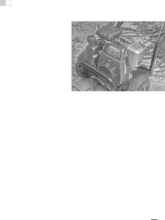
Figure 23.17. An image tonemapped using
gradient-domain compression.
We could therefore compress a high
dynamic range image by attenuating
large gradients, rather than threshold-
ing the gradient field. This approach
was taken by Fattal et al. who showed
that high dynamic range imagery may
be successfully compressed by integrat-
ing a compressed gradient field (Fig-
ure 23.17) (Fattal et al., 2002). Fat-
tal’s gradient-domain compression is
not limited to diffuse scenes.
23.7 Spatial Operators
In the following sections, we discuss tone reproduction operators which apply
compression directly on pixels without transformation to other domains. Often
global and local operators are distinguished. Tone reproduction operators in the
former class change each pixel’s luminance values according to a compressive
function which is the same for each pixel. The term global stems from the fact that
many such functions need to be anchored to some values determined by analyzing
the full image. In practice, most operators use the geometric average
¯
L
v
to steer
the compression:
¯
L
v
=exp
&
1
N
x,y
log(δ + L
v
(x, y)
'
. (23.1)
In Equation (23.1), a small constant δ is introduced to prevent the average to be-
come zero in the presence of black pixels. The geometric average is normally
mapped to a predefined display value. The effect of mapping the geometric aver-
age to different display values is shown in Figure 23.18. Alternatively, sometimes
the minimum or maximum image luminance is used. The main challenge faced
in the design of a global operator lies in the choice of the compressive function.
On the other hand, local operators compress each pixel according to a specific
compression function which is modulated by information derivedfrom a selection
of neighboring pixels, rather than the full image. The rationale is that a bright
pixel in a bright neighborhood may be perceived differently than a bright pixel in
a dim neighborhood. Design challenges in the development of a local operator
involves choosing the compressive function, the size of the local neighborhood
i
i
i
i
i
i
i
i
23.7. Spatial Operators 609
Figure 23.18. Spatial tonemapping operator applied after mapping the geometric average
to different display values (left: 0.12, right: 0.38).
for each pixel, and the manner in which local pixel values are used. In general,
local operators achieve better compression than global operators (Figure 23.19),
albeit at a higher computational cost.
Both global and local operators are often inspired by the human visual sys-
tem. Most operators employ one of two distinct compressive functions, which
is orthogonal to the distinction between local and global operators. Display val-
ues L
d
(x, y) are most commonly derived from image luminances L
v
(x, y) by the
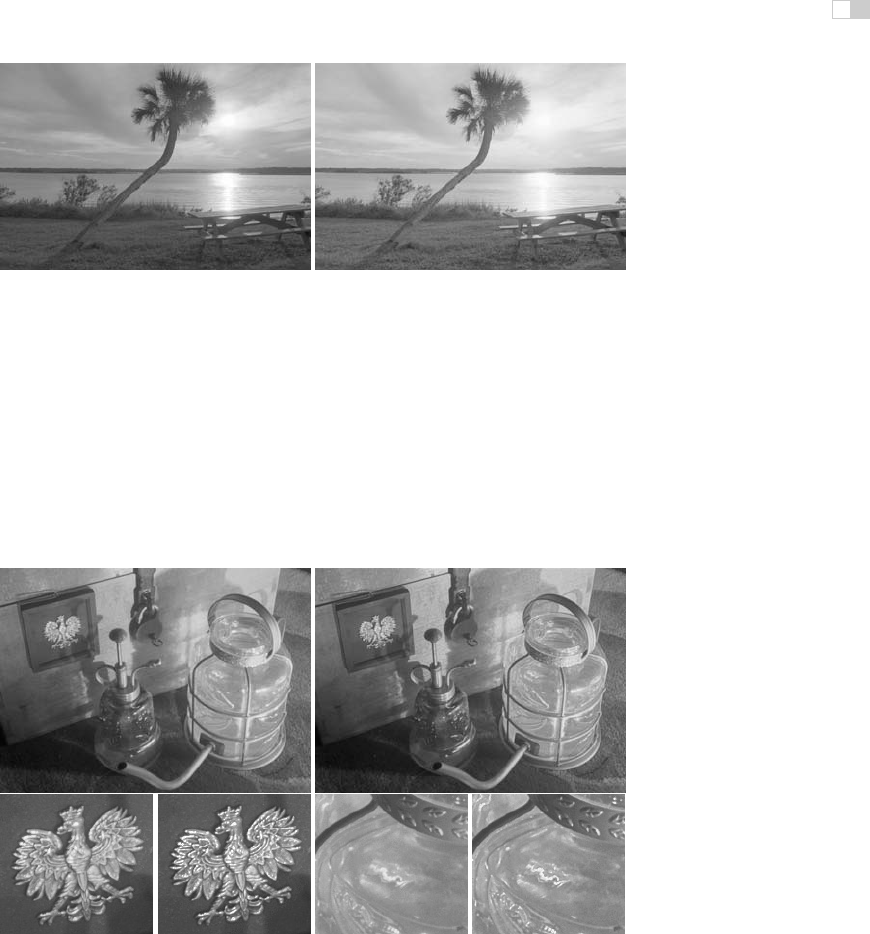
Figure 23.19. A global tone reproduction operator (left) and a local tone reproduction
operator (right) (Reinhard et al., 2002) of each image. The local operator shows more detail;
for example the metal badge on the right shows better contrast and the highlights are crisper.

i
i
i
i
i
i
i
i
610 23. Tone Reproduction
following two functional forms:
L
d
(x, y)=
L
v
(x, y)
f(x, y)
, (23.2)
L
d
(x, y)=
L
v
(x, y)
L
v
(x, y)+f
n
(x, y)
. (23.3)
In these equations, f(x, y) may either be a constant or a function which varies per
pixel. In the former case, we have a global operator, whereas a spatially varying
function f(x, y) results in a local operator. The exponent n is usually a constant
which is fixed for a particular operator.
Equation (23.2) divides each pixel’s luminance by a value derived from either
the full image or a local neighborhood. Equation (23.3) has an S-shaped curve on
a log-linear plot and is called a sigmoid for that reason. This functional form fits
data obtained from measuring the electrical response of photoreceptors to flashes
of light in various species. In the following sections, we discuss both functional
forms.
23.8 Division
Each pixel may be divided by a constant to bring the high dynamic range image
within a displayable range. Such a division essentially constitutes linear scaling,
as shown in Figure 23.3. While Figure 23.3 shows ad-hoc linear scaling, this
approach may be refined by employing psychophysical data to derive the scaling
constant f(x, y)=k in Equation (23.2) (G. J. Ward, 1994; Ferwerda et al., 1996).
Alternatively, several approaches exist that compute a spatially varying di-
visor. In each of these cases, f(x, y) is a blurred version of the image, i.e.,
f(x, y)=L
blur
v
(x, y). The blur is achieved by convolving the image with a
Gaussian filter (Chiu et al., 1993; Rahman et al., 1996). In addition, the computa-
tion of f(x, y) by blurring the image may be combined with a shift in white point
for the purpose of color appearance modeling (Fairchild & Johnson, 2002; G. M.
Johnson & Fairchild, 2003; Fairchild & Johnson, 2004).
The size and the weight of the Gaussian filter has a profound impact on the
resulting displayable image. The Gaussian filter has the effect of selecting a
weighted local average. Tone reproduction is then a matter of dividing each pixel
by its associated weighted local average. If the size of the filter kernel is chosen
too small, then haloing artifacts will occur (Figure 23.20 (left)). Haloing is a com-
mon problem with local operators and is particularly evident when tone mapping
relies on division.
i
i
i
i
i
i
i
i
23.9. Sigmoids 611
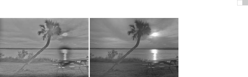
Figure 23.20. Images tonemapped by dividing by Gaussian blurred versions. The size
of the filter kernel is 64 pixels for the left image and 512 pixels for the right image. For
division-based algorithms, halo artifacts are minimized by choosing large filter kernels.
In general, haloing artifacts may be minimized in this approach by making the
filter kernel large (Figure 23.20 (right)). Reasonable results may be obtained by
choosing a filter size of at least one quarter of the image. Sometimes even larger
filter kernels are desirable to minimize artifacts. Note, that in the limit, the filter
size becomes as large as the image itself. In that case the local operator becomes
global, and the extra compression normally afforded by a local approach is lost.
The functional form whereby each pixel is divided by a Gaussian blurred pixel
at the same spatial position thus requires an undesirable tradeoff between amount
of compression and severity of artifacts.
23.9 Sigmoids
Equation (23.3) follows a different functional form from simple division, and,
therefore, affords a different tradeoff between amount of compression, presence
of artifacts, and speed of computation.
Sigmoids have several desirable properties. For very small luminance values,
the mapping is approximately linear, so that contrast is preserved in dark areas of
the image. The function has an asymptote at one, which means that the output
mapping is always bounded between 0 and 1.
In Equation (23.3), the function f(x, y) may be computed as a global con-
stant or as a spatially varying function. Following common practice in electro-
physiology, we call f(x, y) the semi-saturation constant. Its value determines
which values in the input image are optimally visible after tonemapping. In par-
ticular, if we assume that the exponent n equals 1, then luminance values equal
to the semi-saturation constant will be mapped to 0.5. The effect of choosing
different semi-saturation constants is shown in Figure 23.21.
..................Content has been hidden....................
You can't read the all page of ebook, please click here login for view all page.