

i
i
i
i
i
i
i
i
602 23. Tone Reproduction
range images is therefore generally larger as well, although at least one standard
(the OpenEXR high dynamic range file format (Kainz et al., 2003)) includes a
very capable compression scheme.
A different approach to limit file sizes is to apply a tone reproduction operator
to the high dynamic data. The result may then be encoded in JPEG format. In
addition, the input image may be divided pixel-wise by the tonemapped image.
Figure 23.6. Dynamic
range of 2.65 log
2
units.
Figure 23.7. Dynamic
range of 3.96 log
2
units.
Figure 23.8. Dynamic
range of 4.22 log
2
units.
Figure 23.9. Dynamic
range of 5.01 log
2
units.
The result of this division can then be subsampled and stored as a small amount of
Figure 23.10. Dynamic
range of 6.56 log
2
units.
data in the header of the same JPEG image (G. Ward & Simmons, 2004). The file
size of such sub-band encoded images is of the same order as conventional JPEG
encoded images. Display programs can display the JPEG image directly or may
reconstruct the high dynamic range image by multiplying the tonemapped image
with the data stored in the header.
In general, the combination of smallest step size and ratio of the smallest and
largest representable values determines the dynamic range that an image encoding
scheme affords. For computer-generated imagery, an image is typically stored as
a triplet of floating point values before it is written to file or displayed on screen,
although more efficient encoding schemes are possible (Reinhard et al., 2005).
Since most display devices are still fitted with eight-bit D/A converters, we may
think of tone reproduction as the mapping of floating point numbers to bytes such
that the result is displayable on a low dynamic range display device.
The dynamic range of individual images is generally smaller, and is deter-
mined by the smallest and largest luminances found in the scene. A simplistic
approach to measure the dynamic range of an image may therefore compute the
ratio between the largest and smallest pixel value of an image. Sensitivity to out-
liers may be reduced by ignoring a small percentage of the darkest and brightest
pixels.
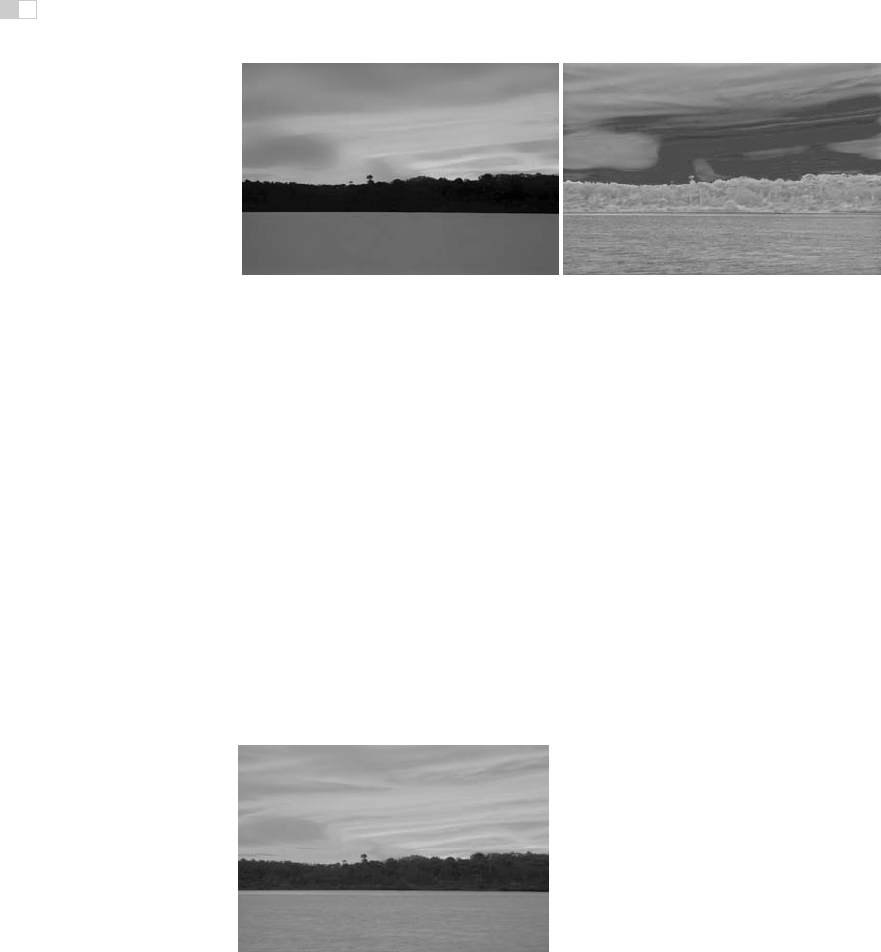
Alternatively, the same ratio may be expressed as a difference in the logarith-
mic domain. This measure is less sensitive to outliers. The images shown in the
margin on this page are examples of images with different dynamic ranges. Note
that the night scene in this case does not have a smaller dynamic range than the
day scene. While all the values in the night scene are smaller, the ratio between
largest and smallest values is not.
However, the recording device or rendering algorithm may introduce noise
which will lower the useful dynamic range. Thus, a measurement of the dynamic
range of an image should factor in noise. A better measure of dynamic range
would therefore be a signal-to-noise ratio, expressed in decibels, as used in signal
processing.

i
i
i
i
i
i
i
i
23.3. Color 603
Figure 23.11. Per-channel gamma correction may desaturate the image. The left image
was desaturated with a value of
s
= 0.5. The right image was not desaturated (
s
= 1). (See
also Plate XIV)
23.3 Color
Tone reproduction operators normally compress luminance values, rather than
work directly on the red, green, and blue components of a color image. Af-
ter these luminance values have been compressed into display values L
d
(x, y),
a color image may be reconstructed by keeping the ratios between color channels
the same as they were before compression (using s =1) (Schlick, 1994b):
I
r,d
(x, y)=
I
r
(x, y)
L
v
(x, y)
s
L
d
(x, y),
I
g,d
(x, y)=
I
g
(x, y)
L
v
(x, y)
s
L
d
(x, y),
I
b,d
(x, y)=
I
b
(x, y)
L
v
(x, y)
s
L
d
(x, y).
The results frequently appear over-saturated, because human color perception is
non-linear with respect to overall luminance level. This means that if we view
an image of a bright outdoor scene on a monitor in a dim environment, our eyes
are adapted to the dim environment rather than the outdoor lighting. By keeping
color ratios constant, we do not take this effect into account.
Alternatively, the saturation constant s may be chosen smaller than one. Such
per-channel gamma correction may desaturate the results to an appropriate level,
as shown in Figure 23.11 and Plate XIV (Fattal et al., 2002). A more compre-
hensive solution is to incorporate ideas from the field of color appearance model-
ing into tone reproduction operators (Pattanaik et al., 1998; Fairchild & Johnson,
2004; Reinhard & Devlin, 2005).
Finally, if an example image with a representative color scheme is already
available, this color scheme may be applied to a new image.Such a mapping of

i
i
i
i
i
i
i
i
604 23. Tone Reproduction
colors between images may be used for subtle color correction such as saturation
adjustment or for more creative color mappings. The mapping proceeds by con-
verting both source and target images to a decorrelated color space. In such a
color space, the pixel values in each color channel may be treated independently
without introducing too many artifacts (Reinhard et al., 2001).
Mapping colors from one image to another in a decorrelated color space is
then straightforward: compute the mean and standard deviation of all pixels in the
source and target images for the three color channels separately.
Figure 23.12. Image used for demonstrat-
ing the color transfer technique. Results are
shown in Figures 23.13 and 23.31. (See
also Plates XV, XVI and XVIII.)
Then, shift and scale the target image
so that in each color channel the mean
and standard deviation of the target im-
age is the same as the source image.
The resulting image is then obtained by
converting from the decorrelated color
space to RGB and clamping negative
pixels to zero. The dynamic range of
the image may have changed as a re-
sult of applying this algorithm. It is
therefore recommended to apply this al-
gorithm on high dynamic range images
and apply a conventionaltone reproduc-
tion algorithm afterwards. A suitable decorrelated color space is the opponent
space from Section 21.2.4.
The result of applying such a color transform to the image in Figure 23.12 is
shown in Figure 23.13.
Figure 23.13. The image on the left is used to adjust the colors of the image shown in
Figure 23.12. The result is shown on the right. (See also Plate XVI.)
i
i
i
i
i
i
i
i
23.4. Image Formation 605
23.4 Image Formation
For now we assume that an image is formed as the result of light being diffusely
reflected off of surfaces. Later in this chapter we relax this constraint to scenes
directly depicting light sources and highlights. The luminance L
v
of each pixel is
then approximated by the following product:
L
v
(x, y)=r(x, y) E
v
(x, y).
Here, r denotes the reflectance of a surface, and E
v
denotes the illuminance. The
subscript v indicates that we are using photometrically weighted quantities. Al-
ternatively, we may write this expression in the logarithmic domain (Oppenheim
et al., 1968):
D(x, y) = log(L
v
(x, y))
= log(r(x, y) E
v
(x, y))
= log(r(x, y)) + log(E
v
(x, y)).
Photographic transparencies record images by varying the density of the material.
In traditional photography, this variation has a logarithmic relation with lumi-
nance. Thus, in analogy with common practice in photography, we will use the
term density representation (D) for log luminance. When represented in the log
domain, reflectance and illuminance become additive. This facilitates separation
of these two components, despite the fact that isolating either reflectance or il-
luminance is an under-constrained problem. In practice, separation is possible
only to a certain degree and depends on the composition of the image. Nonethe-
less, tone reproduction could be based on disentangling these two components of
image formation, as shown in the following two sections.
23.5 Frequency-Based Operators
For typical diffuse scenes, the reflectance component tends to exhibit high spatial
frequencies due to textured surfaces as well as the presence of surface edges. On
the other hand, illuminance tends to be a slowly varying function over space.
Since reflectance is low dynamic range and illuminance is high dynamicrange,
we may try to separate the two components. The frequency-dependence of both
reflectance and illuminance provides a solution. We may for instance compute
the Fourier transform of an image and attenuate only the low frequencies. This
compresses the illuminance component while leaving the reflectance component
i
i
i
i
i
i
i
i
606 23. Tone Reproduction
Figure 23.14. Bilateral filtering removes small details but preserves sharp gradients (left).
The associated detail layer is shown on the right.
largely unaffected—the very first digital tone reproduction operator known to us
takes this approach (Oppenheim et al., 1968).
More recently, other operators have also followed this line of reasoning. In
particular, bilateral and trilateral filters were used to separate an image into base
and detail layers (Durand & Dorsey, 2002; Choudhury & Tumblin, 2003). Both
filters are edge-preserving smoothing operators which may be used in a variety of
different ways. Applying an edge-preserving smoothing operator to a density im-
age results in a blurred image in which sharp edges remain present (Figure 23.14
(left)). We may view such an image as a base layer. If we then pixel-wise divide
the high dynamic range image by the base layer, we obtain a detail layer which
contains all the high frequency detail (Figure 23.14 (right)).
For diffuse scenes, base and detail layers are similar to representations of
illuminance and reflectance. For images depicting highlights and light sources,
Figure 23.15. An image tonemapped using
bilateral filtering. The base and detail layers
shown in Figure 23.14 are recombined after
compressing the base layer.
this parallel does not hold. However,
separation of an image into base and
detail layers is possible regardless of
the image’s content. By compressing
the base layer before recombining into
a compressed density image, a low dy-
namic range density image may be cre-
ated (Figure 23.15). After exponentia-
tion, a displayable image is obtained.
Edge-preserving smoothing opera-
torsmayalsobeusedtocomputealocal
adaptation level for each pixel, which
may be used in a spatially varying or local tone reproduction operator. We de-
scribe this use of bilateral and trilateral filters in Section 23.7.
..................Content has been hidden....................
You can't read the all page of ebook, please click here login for view all page.