

i
i
i
i
i
i
i
i
7
Viewing
In the previous chapter we saw how to use matrix transformations as a tool for
arranging geometric objects in 2D or 3D space. A second important use of geo-
metric transformations is in moving objects between their 3D locations and their
positions in a 2D view of the 3D world. This 3D to 2D mapping is called a viewing
transformation, and it plays an important role in object-order rendering, in which
we need to rapidly find the image-space location of each object in the scene.
When we studied ray tracing in Chapter 4, we covered the different types of
perspective and orthographic views and how to generate viewing rays according
to any given view. This chapter is about the inverse of that process. Here we
explain how to use matrix transformations to express any parallel or perspective
view. The transformations in this chapter project 3D points in the scene (world
space) to 2D points in the image (image space), and they will project any point on
a given pixel’s viewing ray back to that pixel’s position in image space.
If you have not looked at it recently, it is advisable to review the discussion of
perspective and ray generation in Chapter 4 before reading this chapter.
By itself, the ability to project points from the world to the image is only
good for producing wireframe renderings—renderings in which only the edges
of objects are drawn, and closer surfaces do not occlude more distant surfaces
(Figure 7.1). Just as a ray tracer needs to find the closest surface intersection
along each viewing ray, an object-order renderer displaying solid-looking objects
has to work out which of the (possibly many) surfaces drawn at any given point
on the screen is closest and display only that one. In this chapter, we assume we
are drawing a model consisting only of 3D line segments that are specified by
141
i
i
i
i
i
i
i
i
142 7. Viewing
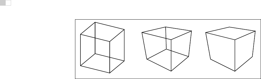
Figure 7.1. Left: wireframe cube in orthographic projection. Middle: wireframe cube in
perspective projection. Right: perspective projection with hidden lines removed.
the (x, y, z) coordinates of their two end points. Later chapters will discuss the
machinery needed to produce renderings of solid surfaces.
7.1 Viewing Transformations
The viewing transformation has the job of mapping 3D locations, represented
as (x, y, z) coordinates in the canonical coordinate system, to coordinates in the
image, expressed in units of pixels. It is a complicated beast that depends on
Some APIs use “viewing
transformation” for just the
piece of our viewing trans-
formation that we call the
camera transformation.
many different things, including the camera position and orientation, the type
of projection, the field of view, and the resolution of the image. As with all
complicated transformations it is best approached by breaking it up in to a product
of several simpler transformations. Most graphics systems do this by using a
sequence of three transformations:
• A camera transformation or eye transformation, which is a rigid body trans-
formation that places the camera at the origin in a convenient orientation.
It depends only on the position and orientation, or pose, of the camera.
• A projection transformation, which projects points from camera space so
that all visible points fall in the range −1 to 1 in x and y. It depends only
on the type of projection desired.
• A viewport transformation or windowing transformation, which maps this
unit image rectangle to the desired rectangle in pixel coordinates. It de-
pends only on the size and position of the output image.
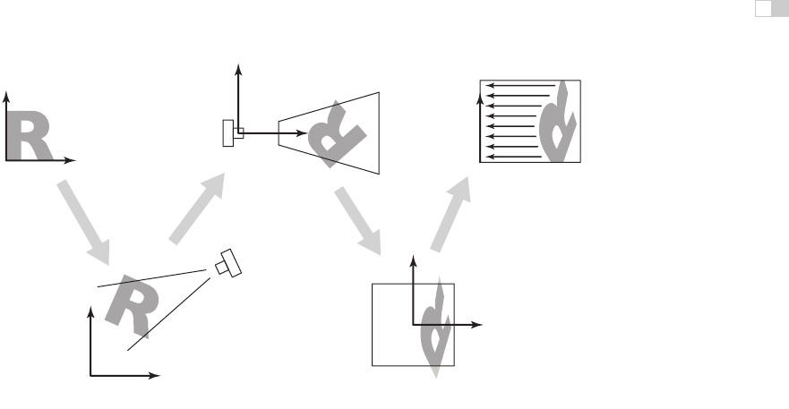
To make it easy to describe the stages of the process (Figure 7.2), we give names
to the coordinate systems that are the inputs and output of these transformations.
The camera transformation converts points in canonical coordinates (or world
i
i
i
i
i
i
i
i
7.1. Viewing Transformations 143
object space
world space
camera space
screen space
modeling
transformation
viewport
transformation
projection
transformation
camera
transformation
canonical
view volume
Figure 7.2. The sequence of spaces and transformations that gets objects from their
original coordinates into screen space.
space) to camera coordinates or places them in camera space. The projection
transformation moves points from camera space to the canonical view volume.
Other names: camera
space is also “eye space”
and the camera transfor-
mation is sometimes the
“viewing transformation;”
the canonical view volume
is also “clip space” or
“normalized device coor-
dinates;” screen space is
also “pixel coordinates.”
Finally, the viewport transformation maps the canonical view volume to screen
space.
Each of these transformationsis individually quite simple. We’ll discuss them
in detail for the orthographic case beginning with the viewport transformation,
then cover the changes required to support perspective projection.
7.1.1 The Viewport Transformation
We begin with a problem whose solution will be reused for any viewing condition.
We assume that the geometry we want to view is in the canonical view volume,
The word “canonical” crops
up again—it means some-
thing arbitrarily chosen for
convenience. For instance,
the unit circle could be
called the “canonical circle.”
and we wish to view it with an orthographic camera looking in the −z direction.
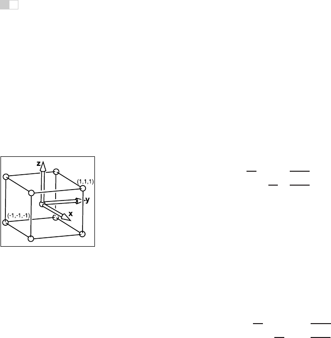
The canonical view volume is the cube containing all 3D points whose Cartesian
coordinates are between −1 and +1—that is, (x, y, z) ∈ [−1, 1]
3
(Figure 7.3).
We project x = −1 to the left side of the screen, x =+1to the right side of the
screen, y = −1 to the bottom of the screen, and y =+1to the top of the screen.
Recall the conventionsfor pixelcoordinates from Chapter 3: each pixel “owns”
a unit square centered at integer coordinates; the image boundaries have a half-
unit overshoot from the pixel centers; and the smallest pixel center coordinates
i
i
i
i
i
i
i
i
144 7. Viewing
are (0, 0). If we are drawing into an image (or window on the screen) that has
n
x
by n
y
pixels, we need to map the square [−1, 1]
2
to the rectangle [−0.5,n
x
−
0.5] × [−0.5,n
y
− 0.5].Mapping a square to a po-
tentially non-square rectan-
gle is not a problem;
x
and
y
just end up with differ-
ent scale factors going from
canonical to pixel coordi-
nates.
For now we will assume that all line segments to be drawn are completely
inside the canonical view volume. Later we will relax that assumption when we
discuss clipping.
Since the viewport transformation maps one axis-aligned rectangle to another,
it is a case of the windowing transform given by Equation (6.6):
⎡
⎣
x
screen
y
screen
1
⎤
⎦
=
⎡
⎣
n
x
2
0
n
x
−1
2
0
n
y
2
n
y
−1
2
00 1
⎤
⎦
⎡
⎣
x
canonical
y
canonical
1
⎤
⎦
. (7.1)
Note that this matrix ignores the z-coordinate of the points in the canonical view
Figure 7.3. The canonical
view volume is a cube with
side of length two centered
at the origin.
volume, because a point’s distance along the projection direction doesn’t affect
where that point projects in the image. But before we officially call this the view-
port matrix, we add a row and column to carry along the z-coordinate without
changing it. We don’t need it in this chapter, but eventually we will need the z
values because they can be used to make closer surfaces hide more distant surfaces
(see Section 8.2.3).
M
vp
=
⎡
⎢
⎢
⎣
n
x
2
00
n
x
−1
2
0
n
y
2
0
n
y
−1
2
001 0
000 1
⎤
⎥
⎥
⎦
. (7.2)
7.1.2 The Orthographic Projection Transformation
Of course, we usually want to render geometry in some region of space other than
the canonical view volume. Our first step in generalizing the view will keep the
view direction and orientation fixed looking along −z with +y up, but will allow
arbitrary rectangles to be viewed. Rather than replacing the viewportmatrix, we’ll
augment it by multiplying it with another matrix on the right.
Under these constraints, the view volume is an axis-aligned box, and we’ll
name the coordinates of its sides so that the view volume is [l, r] × [b, t] × [f,n]
shown in Figure 7.4. We call this box the orthographic view volume and refer to

i
i
i
i
i
i
i
i
7.1. Viewing Transformations 145
the bounding planes as follows:
x = l ≡ left plane,
x = r ≡ right plane,
y = b ≡ bottom plane,
y = t ≡ top plane,
z = n ≡ near plane,
z = f ≡ far plane.
That vocabulary assumes a viewer who is looking along the minus z-axis with
Figure 7.4. The ortho-
graphic view volume.
his head pointing in the y-direction.
1
This implies that n>f,whichmaybe
unintuitive, but if you assume the entire orthographic view volume has negative z
values then the z = n “near” plane is closer to the viewer if and only if n>f;
here f is a smaller number than n, i.e., a negative number of larger absolute value
than n.
This concept is shown in Figure 7.5. The transform from orthographic view
volume to the canonical view volume is another windowing transform, so we can
simply substitute the bounds of the orthographic and canonical view volumes into
Equation (6.7) to obtain the matrix for this transformation:
n
and
f
appear in what
might seem like reverse or-
der because
n–f
, rather
than
f–n
, is a positive num-
ber.
M
orth
=
⎡
⎢
⎢
⎣
2
r−l
00−
r+l
r−l
0
2
t−b
0 −
t+b
t−b
00
2
n−f
−
n+f
n−f
00 0 1
⎤
⎥
⎥
⎦
. (7.3)
Figure 7.5. The orthographic view volume is along the negative
z
-axis, so
f
is a more
negative number than
n
, thus
n
>
f
.
1
Most programmers find it intuitive to have the x-axis pointing right and the y-axis pointing up. In
a right-handed coordinate system, this implies that we are looking in the −z direction. Some systems
use a left-handed coordinate system for viewing so that the gaze direction is along +z. Which is best
is a matter of taste, and this text assumes a right-handed coordinate system. A reference that argues
for the left-handed system instead is given in the notes at the end of the chapter.
..................Content has been hidden....................
You can't read the all page of ebook, please click here login for view all page.