
2 Potential
Problems
2.1 INTRODUCTION
Many engineering problems such as seepage, heat conduction,
electrical problems, etc. are governed by a Laplace or Poisson
equation of the type,
V
2
u = b (2.1)
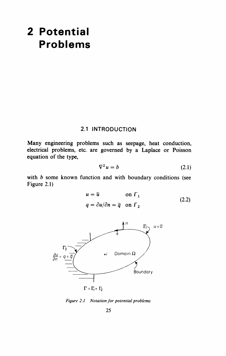
with b some known function and with boundary conditions (see
Figure 2.1)
u = u
onfj
q = du/dn = q on Γ
2
(2.2)
Boundary
r =
r,*r
2
Figure 2.1 Notation for potential problems
25
26 POTENTIAL PROBLEMS
As we have seen, this system can be written as a weighted residual
statement as follows,
- bwdß+ (V
2
u)wdQ = (q-q)xvdr- (u-ü)^dr
(2.3)
Integrating this expression by parts twice we obtain,
- bwdü + {V
2
w)udQ = - qwdr- qwdr +
Jß
Ja Jr
2
Jr
x
Jr
2
3n J
ri
dn
Note that in order to transform the problem into a boundary problem
we need to find a
w
function such that V
2
w = 0 or a
M
function giving
V
2
u
= 0. These approaches leave us with only one domain integral in
terms of b. We can divide the boundary solutions into two types,
(a) Solutions which satisfy the equation V
2
u = 0 in Ω but not the
boundary conditions on Γ. These solutions can be found with
equation (2.3).
(b) Methods for which the weighting function satisfies V
2
w = 0.
The boundary terms need weighting as shown in equation (2.4).
The two methods of solution may be based on approximate
functions that satisfy V
2
( ) = 0 or on a particular type of solution
called the fundamental solution. This is the solution for the Laplace
equation in an infinite domain and with a unit applied potential at a
given point T, i.e.
V
2
«* = St (2.5)
where S
t
is a Dirac delta function representing a unit concentrated
potential acting at a point i. This type of solution is widely used in
boundary problems and represents the Green's or influence function.
Solutions that satisfy V
2
w = 0 have been shown in Chapter 1. We
are now interested in the possibility of using the fundamental solution
to develop a more general method.
..................Content has been hidden....................
You can't read the all page of ebook, please click here login for view all page.