
192 COMBINATION OF REGIONS
In this way a boundary element matrix equation could be obtained in
the way previously shown. The equations can then be superimposed
to the finite element solution for region Ω
χ
and the problem solved
along the lines described in Section 7.2. This approach has been used
by Chen and Mei
5
and more recently by Shaw and Falby.
6
It has the
disadvantage that the boundary values are all interrelated, resulting in
non-banded equations, and that it may be cumbersome to work with
Hankel's functions.
In the conventional boundary element approach the observation
point is taken to be on the boundary. Each observation point gives us
one equation connecting the unknowns du/dn and u, which are
evaluated on the boundary. If, however, we take the observation
points to be in the region Ω
2
far from our problem region we may
make the following important simplification using the asymptotic
forms for the Hankel function, hence
H
M(
K
r)= /_?-
β
χρ[-ί(κτ-π/4)] (7.12)
0 l
' = -ΚΗ[
2)
(ΚΓ)~ -ικ / exp[-i(icr-7E/4)] (7.13)
dn juKr
(note that now n ~ r). Substituting these asymptotic forms into (7.11),
taking Γ to be a large circle of radius R we obtain
2
πκ
e
m/4 ( "
+iK
.
Me
-iKK
)
dr=0
(7.14)
Jr^/R vR J
If
we
now use the fact that R is constant on Γ we can write (7.14) as an
integral over the angular coordinate
Θ
as:
V^(^
+
i
*
M
)
dö
= 0
(7.15)
Note that this
is
just the form of the Sommerfeld radiation condition,
which may be applied approximately on Γ as,
du .
— +
IKM
= 0
(7.16)
or
this condition has been successfully applied in many fluid mechanics
problems. However, the present approach can be extended to develop
COMBINATION OF REGIONS 193
other types of boundary elements, such as those to be used in soil
mechanics problems.
Example 7.2
In order to determine how the application of the above radiation
boundary condition affects the accuracy of
the
solution, the case of a
single vertical column subject to an incident harmonic wave was
studied.
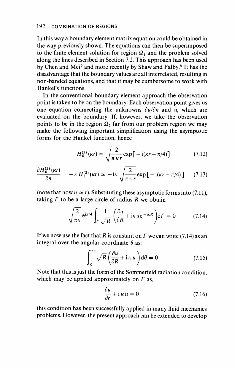
The column was surrounded by a finite element mesh as shown in
(Figure 7.12), and wave diffraction results were found for different
wavelengths, with the application of condition (7.16) on the external
boundary.
161 nodes
» 268 elements
Figure 7.12 Finite element mesh
As a test to determine the adequacy of the radiation condition in
representing a train of plane harmonic waves, the case with no solid
cylinder was studied first. For long waves
(A,
wavelength ~
30 m)
the
results were very accurate, within
3 %
of the exact solution. When the
wavelength
was
reduced the errors tended to increase, which
was
to be
expected
as
the element mesh became too
coarse.
It
was
found that for
194 COMBINATION OF REGIONS
linear elements such as the ones used here, ideally 8 elements per
wavelength should be used.
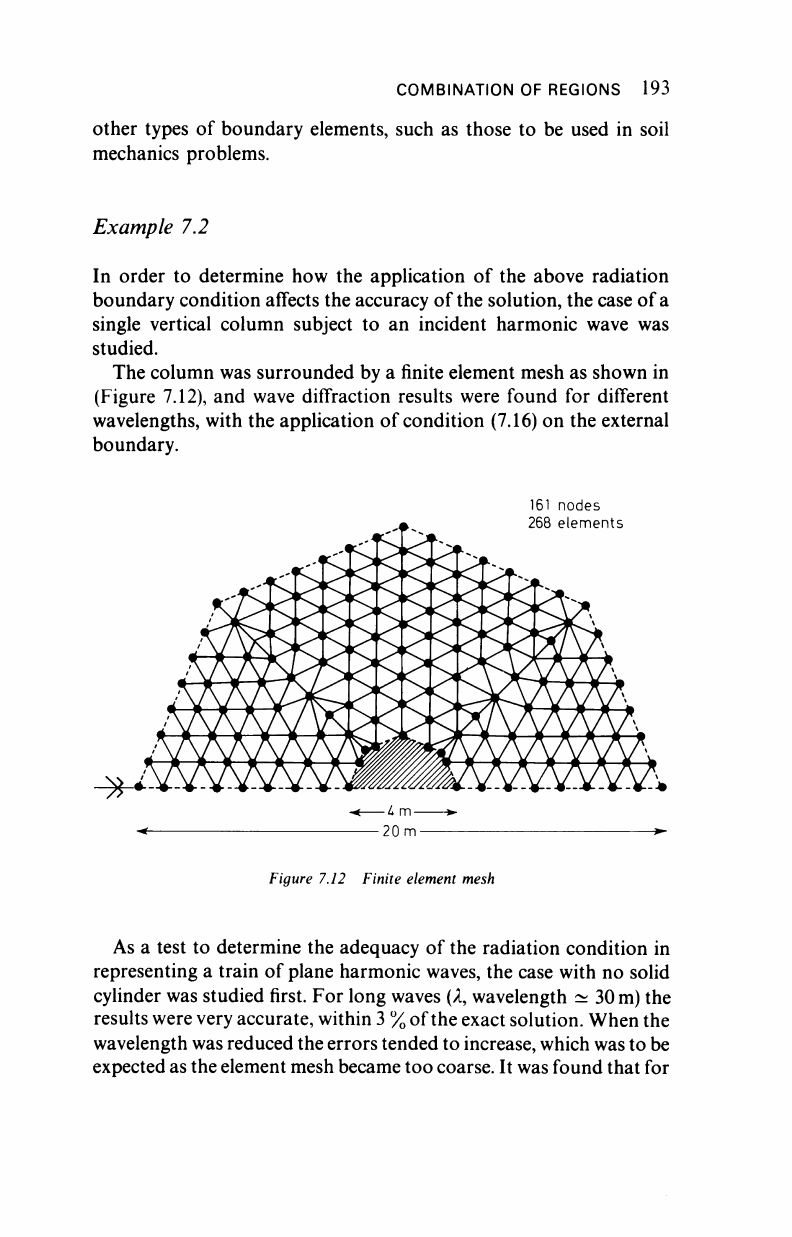
A further test was run to compare our results with those obtained
by Mei
7
using a finite element mesh and the Hankel function
formulation, i.e. the fundamental solution. The results are for an
incident wave with wavelength λ = 2π m and unit incident surface
elevation for frequency ω = 31321. In Figure 7.13 the results of the
exact solution, the finite element solution due to Mei and the solution
obtained by the authors are compared. The present solution (7.9)
compares favourably taking into consideration the coarseness of the
5 c
2 0
1-6
1 2
i
0 8
0-i
0"
.><
//
^ /
Y*-
/
45 90 135
0(deg)
180
Figure 7.13 Results for
maximum
surface elevations round a circular cylinder: radius
= 2
m,
wave length = 2nm. , from Mei
1
; , analytical;
^.authors"
results (coarse mesh with linear interpolation)
mesh around the cyliner. Mei's solution for instance uses 18 elements
round the cyliner and represents the geometry of the obstruction
better.
Example 73 Harbour Resonance*
As another example of the application of this method we will consider
the harbour resonance equation, i.e.
dx dx
(£Κ(£)
+Λ
"-°
COMBINATION OF REGIONS 195
with boundary condition
du
G{u)
= ft— = q on Γ
2
, (b)
on
where
w
is the wave elevation referred to the still water levei with in-
plane coordinates x and y, ft is the depth, q is a given value on Γ
2
boundaries and κ is the wavenumber.
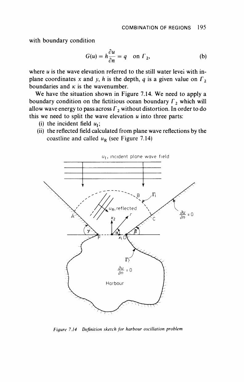
We have the situation shown in Figure 7.14. We need to apply a
boundary condition on the fictitious ocean boundary Γ
2
which will
allow wave energy to pass across Γ
2
without distortion. In order to do
this we need to split the wave elevation u into three parts:
(i) the incident field u
x
(ii) the reflected field calculated from plane wave reflections by the
coastline and called u
R
(see Figure 7.14)
Uj,
incident plane wave field
Figure 7.14 Definition sketch for harbour oscillation problem
196 COMBINATION
OF
REGIONS
(iii)
the
scattered field M
S
originating from inside
the
harbour.
Hence
the
total wave field
is
u
=
u
Y
+ u
R
+ u
s
with
the
incident field given
by
u
x
= a
exp[
—
KY cos
(Θ —
a)]
(c)
(d)
We know that
the
scattered wave field
u
s
will
be
travelling away
from
the
harbour mouth
on Γ
2
.
This fact
is
represented
by the
Sommerfeld boundary condition which
may be
written
lim
r
-►
oo
[s>&*
or approximately
Bus
dr
IKU
S
+ IKU
S
= 0 on Γ
=
0
(e)
(0
using
(f) we may
write
for the
total field
u
—
+
lfCM
= —(M, +
MR)
+
1IC(MI
+ U
R
) = J
(g)
Note that
the
right-hand side
is a
known function/of the horizontal
coordinates,
the
angles determining
the
local geometry
and the
angle
of incidence
of the
wave field
u
x
.
We
may now
incorporate this boundary condition into
our
variational formulation
to
obtain
ΙΙέ(^Κ(*Ι)·
-Ik
du
h
— -q )vdr +
en
r,
νάΩ
h—-
+ 'KU—f
νάΓ
en
(h)
which after integration
by
parts gives
f
/, du dv , du dv ,, ,_
[h
— —
+
h
— —
-K
2
huv
)άΩ
J
ß
ix dx dy dy )
qvdr
+
r
2
(hf—if<hu)vdr
(i)
r,
which
is the
starting expression
for our
finite element formulation
incorporating
the
boundary condition
(f) on Γ.
..................Content has been hidden....................
You can't read the all page of ebook, please click here login for view all page.