
COMBINATION OF REGIONS 201
not give an accurate indication of the behaviour of the system towards
infinity but the effect of the far region on the domain of interest is
introduced (see Bettess
2
).
Example 7.4
10
Diffraction and refraction of waves by a
parabolic shoal, surmounted by a cylindrical island
Figure 7.18 shows the geometry of the problem and the element mesh
used. The finite element mesh is enclosed by a number of infinite
elements, the shape function in the radial direction is given by
P(r)e-^
L
Q-
iKr
(a)
(for time dependence e
lwi
). Here P(r) is a polynomial in r and L is the
so-called decay length, and κ is the wavenumber corresponding to the
frequency ω. This shape function satisfies the Sommerfeld radiation
condition.
L was chosen so that near the island the decay e~
3/L
roughly
matched the decay of the first term of the general series solution,
H
(
0
2)
(/cr), where H
(
0
2)
is the Hankel function of the zeroth order of the
second kind. See Bettess and Zienkiewicz
10
for a fuller explanation of
the above theory.
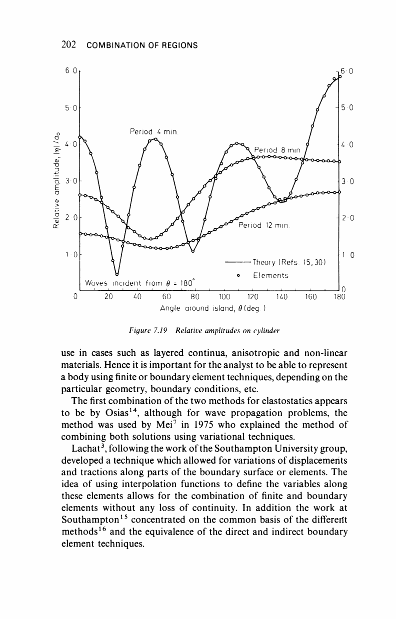
Figure 7.19, from Bettess and Zienkiewicz
10
, shows a comparison
of the elevations at the island itself compared with the analytic
solution given in Homas
1
*
and Vastano and Reid.
12
The agreement is
very good especially at moderate wavelengths.
The weakness in this method is that to determine the parameter L
some knowledge of the exact solution is required before it can be used.
However, the method is very efficient if this information is available.
7.5 COMBINATION OF FINITE AND BOUNDARY ELEMENTS
The idea of combining both techniques can be attributed to Wexler
13
,
who started to use integral equation solutions to represent the
unbounded field problem early in the 1970s, the advantage being that
this allowed for the use of appropriate conditions to represent the
infinite domain. The integral equation technique is also of interest
when regions of high stress or potential gradients exist, but finite
elements are adequate for other parts of a body and may be simpler to
202 COMBINATION OF REGIONS
60 80 100 120
Angle around island,
Θ
(deg )
Figure 7.19 Relative amplitudes on cylinder
use in cases such as layered continua, anisotropic and non-linear
materials. Hence it is important for the analyst to be able to represent
a body using finite or boundary element techniques, depending on the
particular geometry, boundary conditions, etc.
The first combination of the two methods for elastostatics appears
to be by Osias
14
, although for wave propagation problems, the
method was used by Mei
7
in 1975 who explained the method of
combining both solutions using variational techniques.
Lachat
3
, following the work of the Southampton University group,
developed a technique which allowed for variations of displacements
and tractions along parts of the boundary surface or elements. The
idea of using interpolation functions to define the variables along
these elements allows for the combination of finite and boundary
elements without any loss of continuity. In addition the work at
Southampton
15
concentrated on the common basis of the differerit
methods
16
and the equivalence of the direct and indirect boundary
element techniques.
COMBINATION OF REGIONS 203
In this section the combination of boundary and finite elements is
attempted for two-dimensional elastostatic problems and two
dif-
ferent approaches are discussed here.
17
The one that appears more
interesting is that for which the boundary element region is treated as
a finite element, and can thus be easily incorporated into existing finite
element computer packages (see Zienkiewicz, Kelly and Bettess
18
).
The technique is applied to a series of examples to illustrate how the
combination can be done and how accurate the results are.
The starting expression for a finite element elasticity problem is,
I Mfdfi- I o
jk
E%aQ = - I
p
k
u*dr
(7.31)
JQ JQ Jr
2
where wf are the virtual displacements.
The one for boundary elements is,
M?dß +
Ω
^
fj
w
k
dß
= - f
p
k
utdr-
I /vi?dr+ I u
k
p?dr+ I ii
fc
pf dr (7.32)
Jr
2
Jr
x
Jr, Jr
2
where
M?
represents the fundamental solution.
The standard finite element system can be written as
KU = F+D (7.33)
where K is the stiffness matrix for the system, F the equivalent nodal
force vector and D the vector due to body force.
The vector F is obtained by weighting the applied tractions p
k
on
Γ
2
by the interpolation functions used for the displacements, i.e.
ΐΛτρ
= Σ
p
k
utdr
where u
nT
is the vector of nodal virtual displacements for the
complete system. The summation applies over the element sides on
the boundary. Under these conditions we can write F as
F = M P (7.34)
where P is a vector of nodal tractions and where M is a matrix due to
the weighting of the boundary tractions by the interpolation fun-
ctions for the displacements. The exact nature of M can be simply

204 COMBINATION OF REGIONS
explained by considering the term
I P
k
utdr (7.35)
in equation (7.31), which is the boundary tractions weighted by the
virtual displacements, or may be interpreted as the external energy
expended due to a virtual displacement u*. For a particular element,
T, pj is a row vector containing the nodal value of the tractions andujf
a column vector containing the arbitrary virtual displacements u*.
(7.35) may now be written as
u*^p
k
dr
(7.36)
Jr,
Assuming the interpolation functions for u and p as
ιι? =
Φιι?·
η
Ρ,= Ψρ
η
(7.37)
The above term reduces to
M
*n,T|
<J>ipT
dr
j
p
n (7.38)
The matrix M may then be expressed as defined in equation (7.33).
Hence we can write (7.32) as
KU = MP+D
which is similar form to the boundary element equation, resulting
from (7.32)
HU = GP+B (7.39)
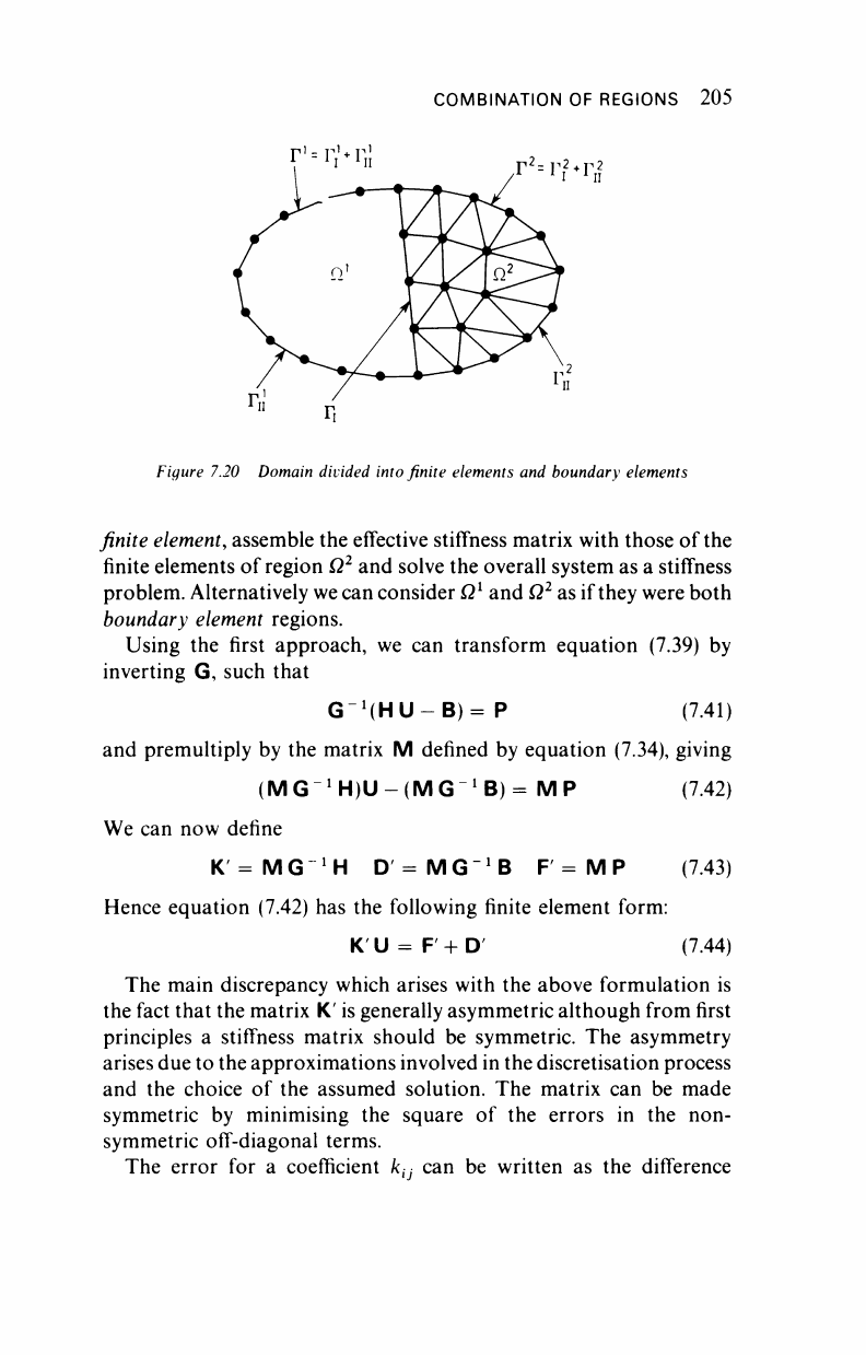
Consider a problem consisting of two domains Ω
1
, Ω
2
joined by an
interface Γ
1
, and which makes use of a finite element formulation in
Ω
2
and a boundary element formulation in Ω
1
(Figure 7.20). In order
to join the two parts we apply compatibility and equilibrium
conditions along the interface Γ
1
, i.e.
U,
1
= U
2
P/ + P
2
= 0 (7.40)
where J,
P[
refer to the displacements and tractions on the interface
Tj for the region /(/ = 1,2 for a two-dimensional problem).
We now have two alternatives as to how to approach the problem.
We may develop the boundary element region Ω
1
as an equivalent
COMBINATION OF REGIONS 205
Figure 7.20 Domain divided into finite elements and boundary elements
finite element, assemble the effective stiffness matrix with those of the
finite elements of region Ω
2
and solve the overall system as a stiffness
problem. Alternatively we can consider Ω
1
and Ω
2
as if they were both
boundary element regions.
Using the first approach, we can transform equation (7.39) by
inverting G, such that
G
!
(HU-B)= P (7.41)
and premultiply by the matrix M defined by equation (7.34), giving
(MG"
1
H)U-(MG
1
B)= MP (7.42)
We can now define
K'=MG
_1
H D'=MG
_1
B F = M P (7.43)
Hence equation (7.42) has the following finite element form:
K U = F + D (7.44)
The main discrepancy which arises with the above formulation is
the fact that the matrix K' is generally asymmetric although from first
principles a stiffness matrix should be symmetric. The asymmetry
arises due to the approximations involved in the discretisation process
and the choice of the assumed solution. The matrix can be made
symmetric by minimising the square of the errors in the non-
symmetric off-diagonal terms.
The error for a coefficient /c
(J
can be written as the difference
..................Content has been hidden....................
You can't read the all page of ebook, please click here login for view all page.