
50 POTENTIAL PROBLEMS
component on the boundary, i.e.
du du
q =
k
*dx
nx
+
k2
eY
nY
(2.90)
This expression allows us to calculate the value of
q
at any point on the
boundary. The formula also applies when u is substituted by the
fundamental solution u*.
2.7 THE HELMHOLTZ EQUATION
Let us now consider the Helmholtz equation, i.e.
V
2
M + /1
2
W = 0
(2.91)
where λ
2
is a positive constant. The boundary conditions are assumed
to be
u= ü on Γ
du/dn = q = q on Γ
2
The starting weighted residual statement for this case is,
(2.92)
(Sl
2
u + X
2
u)u*dQ
(q-q)u*dr
-
(u-ü)q*dr (2.93)
'^1
Integrating twice by parts we obtain,
f
Jß
(V
2
w* + *
2
w*)Mdß =
qu*dr +
q*udr
(2.94)
where Γ = Γ
1
+ Γ
2
. u* is the fundamental solution for the Helmholtz
equation, which satisfies
V
2
M* + A
2
W*+(5
1
=0
For two dimensions this fundamental solution is
1
(2.95)
and
u*=
+-H
(
0
2)
(/ir)
4i
6
f=-i»^
(2.96)
POTENTIAL PROBLEMS 51
r is the distance from the source point to the point under con-
sideration.
H
{
Q
]
is a Hankel function of
the
second kind of zero order,
i.e.
Η^(λτ) = 3
0
(λτ)-Υ
0
(λτ) (2.97)
where J
0
is a Bessel function of the first kind and Y
0
is one of the
second kind. The Hankel function of order one is
H[
2)
(kr)
= J, (λή - i Y, (λή (2.98)
For three dimensions, the fundamental solution is,
u* = e~
Ur
4nr
and (2.99)
du*
1 /l .„ .
or 4nr
Substituting (2.93) into (2.92) we obtain,
u,+
l·
q*dr =
qu*dr (2.100)
If the point
Ί"
is taken to be on the smooth Γ boundary, we will have
for two and three dimensions the following result:
iu,+ uq*dr = qu*dr (2.101)
In general we can write a constant c, instead of for a non-smooth
boundary. Hence,
0^ +
=
l·"
uq*dr = qu*dr (2.102)
From now on the usual boundary element matrix technique can be
applied.
Let us now consider how the solution behaves at infinity by
assuming that we have two boundaries, one
a
closed boundary and the
other the one at infinity (Figure 2.12). Formula (2.102) can now be
written as
CM+ I (uq*-qu*)dr= | (qu*-q*u)dr (2.103)
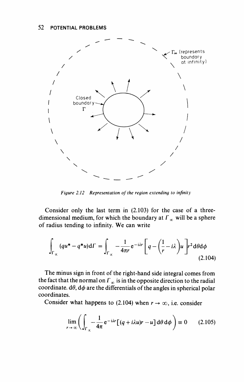
52 POTENTIAL PROBLEMS
/
^Γοο (represents
boundary
at infinity)
Closed
boundary
Γ
/
Figure 2.12 Representation of
the
region extending to infinity
Consider only the last term in (2.103) for the case of a three-
dimensional medium, for which the boundary at Γ
χ
will be a sphere
of radius tending to infinity. We can write
(qu*
—
q*u)dr =
1
Anr
-kr
H->]
Υ
2
άθάφ
(2.104)
The minus sign in front of the right-hand side integral comes from
the fact that the normal on Γ ^ is in the opposite direction to the radial
coordinate, dö, άφ are the differentials of the angles in spherical polar
coordinates.
Consider what happens to (2.104) when r
-►
oo, i.e. consider
lim
r-»·
(X)
- ^-e-
Ur
[(i + i/lu)r -ΐί~άθάφ ) = 0 (2.105)
4π
..................Content has been hidden....................
You can't read the all page of ebook, please click here login for view all page.