
TIME-DEPENDENT AND NON-LINEAR PROBLEMS 173
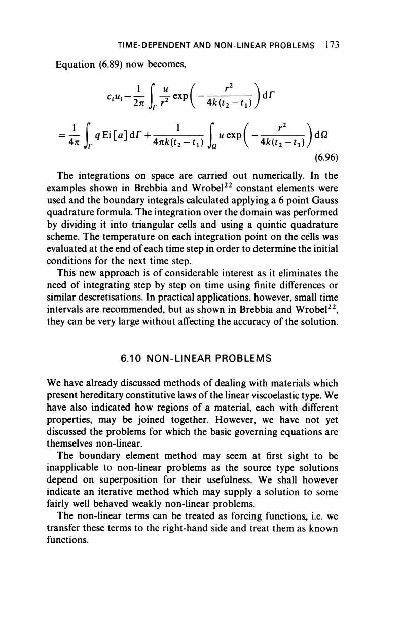
Equation (6.89) now becomes,
(6.96)
The integrations on space are carried out numerically. In the
examples shown in Brebbia and Wrobel
22
constant elements were
used and the boundary integrals calculated applying a 6 point Gauss
quadrature formula. The integration over the domain was performed
by dividing it into triangular cells and using a quintic quadrature
scheme. The temperature on each integration point on the cells was
evaluated at the end of each time step in order to determine the initial
conditions for the next time step.
This new approach is of considerable interest as it eliminates the
need of integrating step by step on time using finite differences or
similar descretisations. In practical applications, however, small time
intervals are recommended, but as shown in Brebbia and Wrobel
22
,
they can be very large without affecting the accuracy of the solution.
6.10 NON-LINEAR PROBLEMS
We have already discussed methods of dealing with materials which
present hereditary constitutive laws of
the
linear viscoelastic type. We
have also indicated how regions of a material, each with different
properties, may be joined together. However, we have not yet
discussed the problems for which the basic governing equations are
themselves non-linear.
The boundary element method may seem at first sight to be
inapplicable to non-linear problems as the source type solutions
depend on superposition for their usefulness. We shall however
indicate an iterative method which may supply a solution to some
fairly well behaved weakly non-linear problems.
The non-linear terms can be treated as forcing functions, i.e. we
transfer these terms to the right-hand side and treat them as known
functions.
174
TIME-DEPENDENT
AND
NON-LINEAR
PROBLEMS
Consider the equation,
^(w) + yT(u) = & (6.97)
where here if is a linear operator, yKis a non-linear operator and & is
some known forcing function.
The iterative procedure will consist of writing (6.97) as,
JS?(II)=
0>-rfu) (6.98)
making some realistic guess for the initial form of
w,
u
0
(or in some
cases taking u
0
= 0). and putting this in the non-linear terms on the
right-hand side, i.e.
&(u
x
) = 0>-JT(
Uo
) (6.99)
If (6.99) is then solved for u
l
in the usual way we may repeat the
process until some criterion for convergence is satisfied. The funda-
mental solution needed for our boundary element formulation when
$£ is self-adjoint is defined by,
JSP(M*)
= S
t
(6.100)
The resulting matrices for the boundary element formulation
will be
HU = GQ+P+N (6.101)
where P represents the body force Vector and N is the vector obtained
from the non-linear terms.
One important feature of this approach is that the influence
matrices H and G remain the same for each iteration. We only need to
recalculate the vector N and find the new solution vector U and Q for
each iteration.
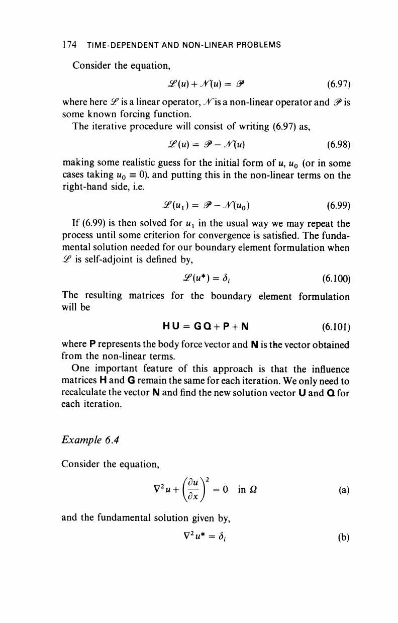
Example 6.4
Consider the equation,
V2
"
+
(S)
2
= 0
ιηΩ
and the fundamental solution given by,
V
2
M*
= <5
;
(a)
(b)
..................Content has been hidden....................
You can't read the all page of ebook, please click here login for view all page.