
6 Time-Dependent
and Non-Linear
Problems
6.1 INTRODUCTION
Up to now we have been considering time-independent problems;
many situations of physical interest involve the solution of problems
with some time component, be it a vibration problem where a steady
state solution is sought, the solution to a problem where the response
to some transient effect is required or the case where the properties of
the material itself are time dependent.
Previous analyses of time-dependent problems using the boundary
element method have been solved by either integrating numerically in
time in some finite difference fashion or by eliminating the time
variation by the use of a Laplace transform
1,2
-
3
-
4
, notably Cruse.
1
The analysis of a simple vibrational problem has been attempted by
Hutchinson
5
effectively, though not explicitly, using the Fourier
decomposition method.
In this chapter the relatively unexplored topic of
the
application of
boundary elements to problems with both material and certain types
of geometric non-linearities will also be discussed. The final section
will include a discussion of the recent applications of boundary
elements to plasticity problems.
6
6.2 TRANSFORM METHODS
In many time-dependent problems involving governing equations
which are linear in the time variable and have time-independent
151
152 TIME-DEPENDENT AND NON-LINEAR PROBLEMS
coefficients it is possible to remove the time dependence in the
equations by taking a Laplace (L) or Fourier transform (&). The
resulting equations may then be solved in the transform space with
the usual boundary element method. Equations involving the time
variable are usually hyperbolic (or parabolic) in type and as such are
unsuitable for solution by the boundary element technique, the
transformed equations, however, are in many cases elliptic.
Once the equations are solved in the transformed space the original
variable involving the time dependence may be recovered by inverting
the transformation numerically. The type of transform used, either
Laplace
(L)
or Fourier (&) will depend on the type of solution sought.
We shall illustrate this point by considering
a
simple 'forced vibration'
problem.
Consider the second-order differential equation,
a
2
u du ,
m
—-=-
+
c —-
+
ku
= Fe^
at
2
at
(6.1)
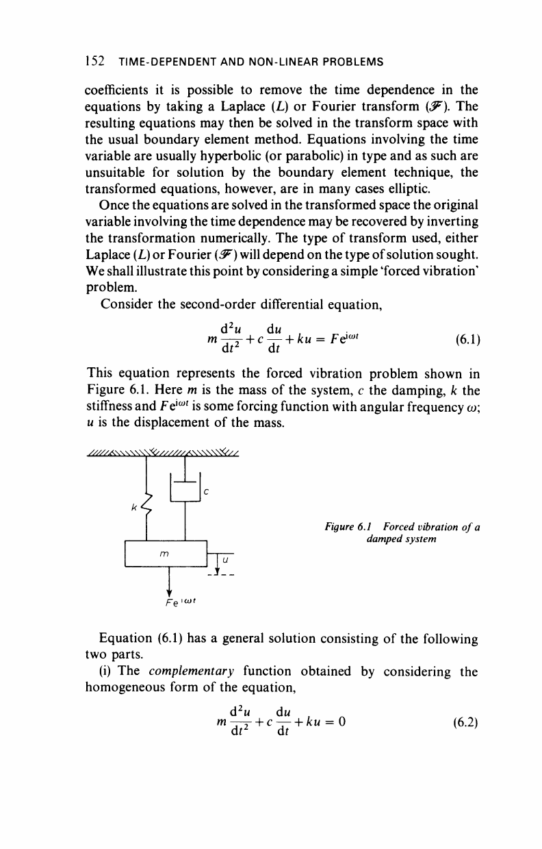
This equation represents the forced vibration problem shown in
Figure 6.1. Here m is the mass of the system, c the damping, k the
stiffness and Fe
lwi
is some forcing function with angular frequency ω;
u is the displacement of the mass.
ζ
Figure 6.1 Forced vibration of a
damped system
Y.
Fe
1
Equation (6.1) has a general solution consisting of the following
two parts.
(i) The complementary function obtained by considering the
homogeneous form of the equation,
d
2
w dw ,
m—-y + c—- +
ku
= 0
at
2
at
(6.2)
TIME-DEPENDENT AND NON-LINEAR PROBLEMS 153
This solution is given by,
u = ,4e
a+i
+ £e
a
' (6.3)
where
c Jc
2
—
4m
"*--2^-2^-
(6
·
4)
A and B are constants determined by the initial displacement u
0
and
velocity ii
0
. By considering u and its time derivative at time t = 0, we
find that
A = and B =
0L+—
a_ a_— a +
This is the 'transient' part of the solution. In general we shall use the
Laplace transform to obtain solutions of this kind.
(ii) The particular integral or solution obtained by postulating a
solution of the type,
u = U έ
ωί
(6.5)
This solution corresponds to a motion with the same frequency as the
forcing function and for a stable system will be the 'steady state'
response to the forcing function Fe*^. This eventual steady state will
be independent of the initial values u
0
and ti
0
.
For our equation this solution is given by
U = 2—
1
-, F (6.6)
— a>
z
m
+
icoc
+ k
We see that U depends on the exciting frequency ω and the properties
of
the
system
m,
c and
k.
In general we shall use the Fourier transform
to obtain solutions of this kind.
The general solution of (6.1) is hence
a+—
a_ a_
—
a+
— ω m
+
a>c
+
k
where a
+
and a_ are given by (6.4).
..................Content has been hidden....................
You can't read the all page of ebook, please click here login for view all page.