
156 TIME-DEPENDENT AND NON-LINEAR PROBLEMS
2,.
. . , N -
1
and
(6.8) may
be
represented approximately
by
1
N
~
l
Γ
Fk
= j Σ
fr
QX
P
-*
where
At = T/N and t = rAt
substituting
T = N At
into (6.16)
gives,
F
k
= ^ Σ
/
r
e-^/
N
fc = 0, 1, 2,. . . ,
JV
-
1
(6.17)
hence
the
inverse discrete Fourier transform
is
given
by
fr
= Σ
F
kC
iü)r/N
r = 0, 1, 2, . . . , N -
1
(6.18)
k = 0
By the use
of
the fast Fourier transform algorithm these calculations
may be considerably simplified
in
the computer, making the process
very efficient
for
evaluating integrals
of the
form given
by (f) in
Example 6.1.
8
6.4 LAPLACE TRANSFORMS
10
This
is
closely related
to the
Fourier transform
but
generally with
some important differences.
If f(t) is a
piecewise differentiable
function with
a
finite number
of
finite discontinuities we may define
the Laplace transform F(K) of fit)
by
F(K)
= L[f(t)-] = fV(i)e-K<di
(6.19)
f(t) is conventionally regarded as zero for
t <
0. We shall indicate that
we are working with the Laplace rather than the Fourier transform by
using
K
as the transform variable in our transformed function
F.
Note
that K may
be
complex and
F (κ)
is
defined
in the
first instance
for
Re(fc)
> y
Where
y is
some constant defined
for
convergence
of
the
integral (6.19) and Re means we take the real part. By integration
by
parts
we
can show that
H
At
(6.16)
TIME-DEPENDENT AND NON-LINEAR PROBLEMS 157
L[df/dt] =
K
F(K)-f(0) (6.20)
where /(0)
is
f(t) evaluated at t = 0.
SimilaHv,
L[d
2
f/dt
2
] =
K
2
F
(K)
-
Kf(0)
-f(0) (6.21)
where /'(0) is df/dt evaluated at t = 0.
Using
(6.20) we may
find
the Laplace transform of
an
integral of/(i)
such that,
We shall also use the 'shifting theorem' which states that
£[e
e
7(0]= /(f)e<
fl
-*>dt = F(ic-a) (6.23)
Hence we have the important result that
L[e
ei
] = —— and L[ie
ei
] =
/
{
. (6.24), (6.25)
κ-α (κ-αΥ
This result will be important when we carry out the numerical
inversion of the Laplace transform.
As an
analogy
with (6.13) one can also
define
a Laplace
convolution
by,
f*9=
Γ/(ί-τ)0(τ)ατ (6.26)
Thus,
L[f*g-] =
F(K)G(K)
(6.27)
where,
F(K)
= L[/m
G(K)
= L[g(t)] (6.28)
Before considering the problems of the inversion of the Laplace
transform, we shall consider its use in the solution of the simple
second-order differential equation with constant coefficients dis-
cussed in Example 6.1.
158 TIME-DEPENDENT AND NON-LINEAR PROBLEMS
Example 6.2
Consider the equation
d
2
u du
dr di
m
^ +
c
^7 +
ku
=f(
t
) (
a
)
now with the initial conditions u(0) = u
0
, ύ(0) = ύ
0
.
If we now take the Laplace transform of this equation we obtain,
mK
2
U{κ)
—
mKU
0
—
mu
0
+
CKU(κ)
—
cu
0
+ k
U(K)
= F(K) (b)
Hence,
U{K) = γ- — (c)
πικ
+CK
+ k
u(t) may then be obtained by using tables of transforms, by analytical
evaluation of the Bromwich inversion integral or by a numerical
inversion process.
Note that the initial values are taken into account in equation (c),
which gives the 'transient' part of the solution.
THE BROMWICH INTEGRAL
We have,
F(
K
)= I e-*'/(t)dr (6.29)
Jo
where Re(K) > y for convergence.
(K) =
Jo
Then the use of Planchard's theorem gives'
9
f(t) =
Q
Kt
F(K)dK (6.30)
This is the Bromwich integral (see Figure 6.2). y
1
is chosen to be
such that equation (6.30) gives/(i) = 0 for t < 0. In fact y
x
is chosen
such that all the singularities of
F (κ)
lie to the left of the contour from
y
l
—
iootoyj+ioo.Bya minor distortion of the contour we may write
(for t > 0),
f(t) =
Y
j
e«j<F
j
(K)
(6.31)
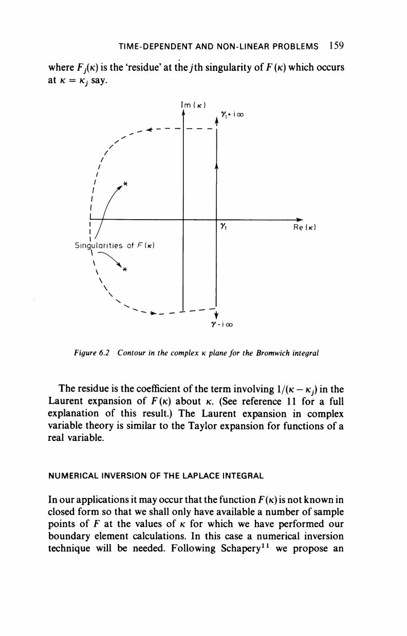
TIME-DEPENDENT AND NON-LINEAR PROBLEMS 159
where
FJ(K)
is the 'residue' at the;th singularity of
F(K)
which occurs
at K = Kj say.
ImU)
Singularities of F{K)
7,+ ioo
Re(ic)
y-ioo
Figure 6.2 Contour in the complex κ plane for the Bromwich integral
The residue is the coefficient of the term involving l/(/c -
Kj)
in the
Laurent expansion of F(K) about κ. (See reference 11 for a full
explanation of this result.) The Laurent expansion in complex
variable theory is similar to the Taylor expansion for functions of a
real variable.
NUMERICAL INVERSION OF THE LAPLACE INTEGRAL
In our applications it may occur that the function
F(K)
is not known in
closed form so that we shall only have available a number of sample
points of F at the values of κ for which we have performed our
boundary element calculations. In this case a numerical inversion
technique will be needed. Following Schapery
11
we propose an
..................Content has been hidden....................
You can't read the all page of ebook, please click here login for view all page.