
198 COMBINATION OF REGIONS
0
15 0 20
0?5
Frequency, o>(rad s"
1
)
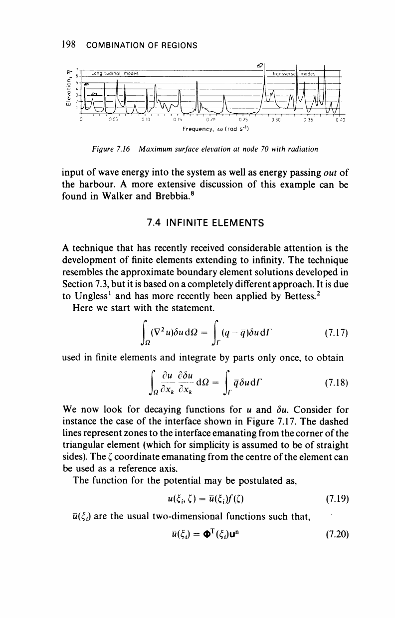
Figure 7.16 Maximum surface elevation at node 70 with radiation
input of wave energy into the system as well as energy passing out of
the harbour. A more extensive discussion of this example can be
found in Walker and Brebbia.
8
7.4 INFINITE ELEMENTS
A technique that has recently received considerable attention is the
development of finite elements extending to infinity. The technique
resembles the approximate boundary element solutions developed in
Section
7.3,
but it is based on
a
completely different approach. It is due
to Ungless
1
and has more recently been applied by Bettess.
2
Here we start with the statement.
{S/
2
u)ouaQ= (q-q)öudr (7.17)
used in finite elements and integrate by parts only once, to obtain
du döu
JQ
dx
k
L
dx
h
dx
k
άΩ =
qöudr
(7.18)
We now look for decaying functions for u and du. Consider for
instance the case of the interface shown in Figure 7.17. The dashed
lines represent zones to the interface emanating from the corner of the
triangular element (which for simplicity is assumed to be of straight
sides).
The ζ coordinate emanating from the centre of
the
element can
be used as a reference axis.
The function for the potential may be postulated as,
ΰ(ξ,) are the usual two-dimensional functions such that,
ΰ(ξι) = Φ
Τ
(^)υ
η
(7.19)
(7.20)
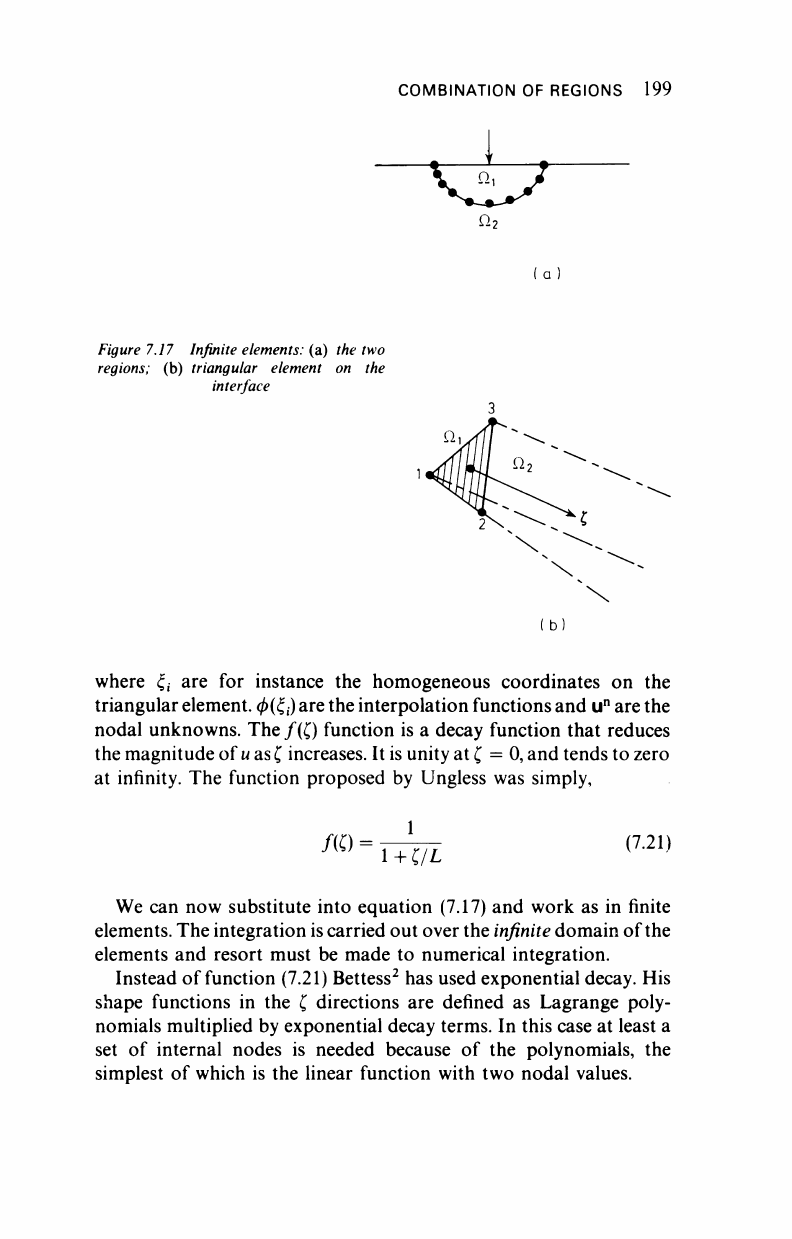
COMBINATION OF REGIONS 199
Figure 7.17 Infinite elements: (a) the two
regions; (b) triangular element on the
interface
:t>)
where ξ
ί
are for instance the homogeneous coordinates on the
triangular element. φ(ξ
ί
) are the interpolation functions and u
n
are the
nodal unknowns. The /(£) function is a decay function that reduces
the magnitude of
u
as ζ increases. It is unity at ζ = 0, and tends to zero
at infinity. The function proposed by Ungless was simply,
/(i)
= TTc/Z
(7
·
21
>
We can now substitute into equation (7.17) and work as in finite
elements. The integration is carried out over the infinite domain of the
elements and resort must be made to numerical integration.
Instead of function (7.21) Bettess
2
has used exponential decay. His
shape functions in the ζ directions are defined as Lagrange poly-
nomials multiplied by exponential decay terms. In this case at least a
set of internal nodes is needed because of the polynomials, the
simplest of which is the linear function with two nodal values.
200 COMBINATION OF REGIONS
The form of the solution will depend on the coefficients taken for
the exponential decay, i.e. on the L of the following equation:
/(C) = F(C)e-^
L
(7.22)
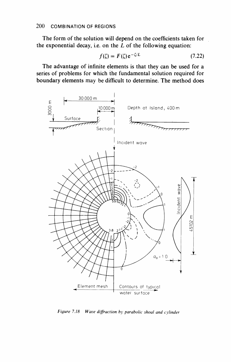
The advantage of infinite elements is that they can be used for a
series of problems for which the fundamental solution required for
boundary elements may be difficult to determine. The method does
o
30 000
m
,10000m Depth at Island, 400 m
I Surface t ■ A
—
=777
| >77Ύ?
Figure 7.18 Wave diffraction by parabolic shoal and cylinder
..................Content has been hidden....................
You can't read the all page of ebook, please click here login for view all page.