
POTENTIAL PROBLEMS 27
2.2 THE FUNDAMENTAL SOLUTION AND DIRECT
FORMULATION
The solution corresponding to an applied potential concentrated at a
point is frequently used in boundary problems. For the Laplace's
equation for instance the fundamental solution that will be called w*
(the asterisk is used to indicate its special character) is the one
corresponding to the following equation:
V
2
w* = S
t
(2.6)
or more explicitly
V
2
u*
= S(x-x
i
) (2.7)
where ö
t
is the Dirac delta function.
Note that this function u* is a function of two points: the 'source'
point
X;
at which we have the singularity of our delta function; and the
'observation' point
3c
which is the variable involved in our differential
equation.
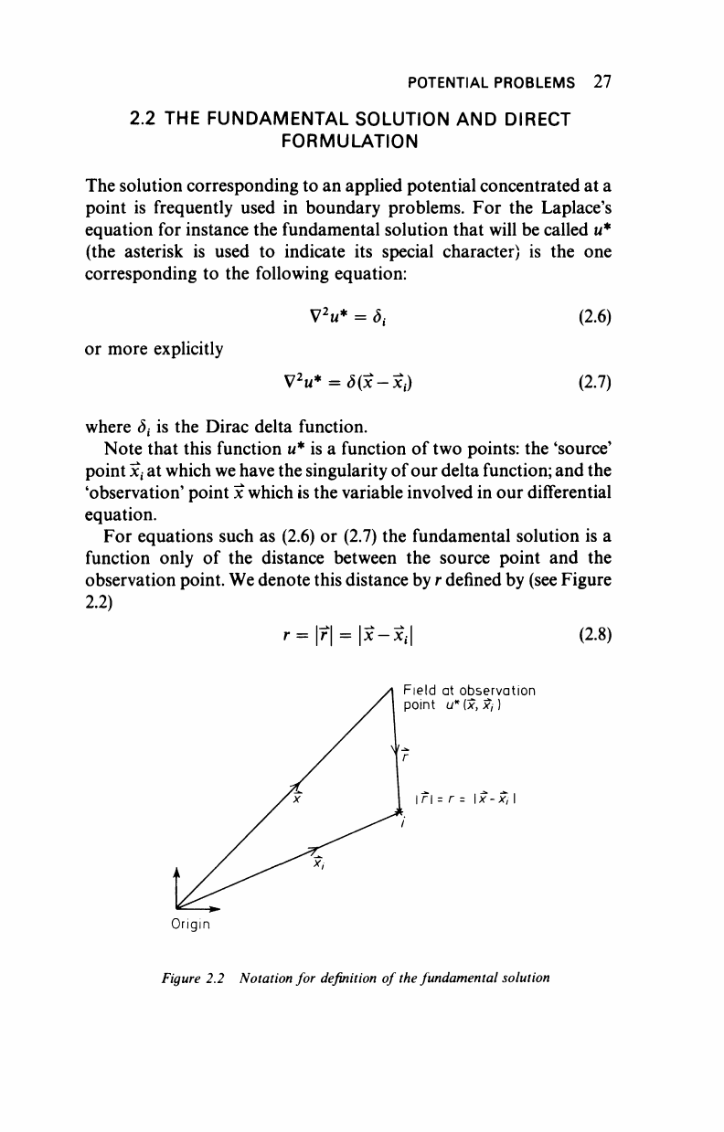
For equations such as (2.6) or (2.7) the fundamental solution is a
function only of the distance between the source point and the
observation point. We denote this distance by r defined by (see Figure
2.2)
r=
= x-Xi (2.8)
Field at observation
point
u*{x,Xj
Origin
Figure 2.2 Notation for definition of
the
fundamental solution
28 POTENTIAL PROBLEMS
This function when weighted
by
any other function
u,
has the
following property:
(V
2
u*)udQ=
dM^ =
^i
(
2
·
9
)
2
}Q
w
t
represents the value
of
the unknown function u
at
the point
of
application
of
the potential.
The fundamental solution
of
equation
(2.6) for a
three-
dimensional isotropic medium is,
V
2
w*
=
1/4*7 (2.10)
We can show that (2.10)
is
the fundamental solution required
by
considering equation (2.6) in spherical polar coordinates.
The field due
to a
point source in isotropic space will only be
a
function of the radial coordinate r, taken to be the distance from the
source, hence we can write
d
2
u*
2
du*
+
+a
0
= 0
(in)
or
r or
without loss of generality we have now taken the source point to be at
the origin. Substituting (2.10) into (2.11) we can easily verify that
(2.10) satisfies the governing equation for any r different from zero. At
r
= 0 a
singularity occurs and we have
to
consider
a
small sphere
surrounding the point i where the load is applied and integrate over it
to find out what will occur when r
-►
0.
This can be done by using Gauss' theorem in the form
l
e
v2
"*
dß=
l^
dr
(2i2)
where O
e
, T
e
are
the volume and surface of the sphere surrounding the
source point. Substituting (2.10) into (2.12) we obtain,
or
4π
l
Jr
1
/4πΓ
2
?)
ar
^-Vn^-)
r
=-
H2
-
U)
Note that this result
is
independent
of
r, hence when r
-►
0, the
integral of
the
potential over the sphere tends to 1. We have therefore
represented
a
unit source strength.
POTENTIAL PROBLEMS
29
The fundamental solution for the isotropic two-dimensional case is
"*-έ'"(;)
,ll4
>
and has similar properties to the three-dimensional case.
If
we
assume that the weighting function is composed of a series of
fundamental solutions applied over the boundary we can work with
equation (2.4). Conversely if the approximating function is assumed
to be a combination of fundamental solutions, equation
(2.3)
could be
used. (Both functions can also
be
taken
to be
combinations
of
fundamental solutions as in the case w
=
Au.)
For the first case we can consider a particular point T for which
u*
is the fundamental solution due to an applied potential acting at that
point. This equation can be written as,
- bu*dQ + (V
2
w*)udß+ qu*dr+ qu*dr
Ja
JQ Jr
2
Jr
l
üq*dr+ uq*dr
(2.15)
where q*
=
du*/dn.
Taking into consideration that at T the governing equation for
u*
is
V
2
«*
=
S
t
(2.16)
Formula (2.15) for the point
'f
under consideration becomes,
ιι,.-h bu*dQ+ uq*dr+ uq*dr= qu*dr
Jß
Jr
2
Jr
l
Jr
2
+
qu*dr (2.17)
This equation relates the value of
u
at the point T with the values of
q
and
u
over the boundary Γ (Figure 2.1). It appplies when the point T is
in the interior domain Ω, but in order to formulate the problem in
terms
of
boundary integrals we need
to
take the point
T to the
boundary. We will now do this analytically for
a
smooth boundary
though we will later on see that we do not need to know the analytical
expression.
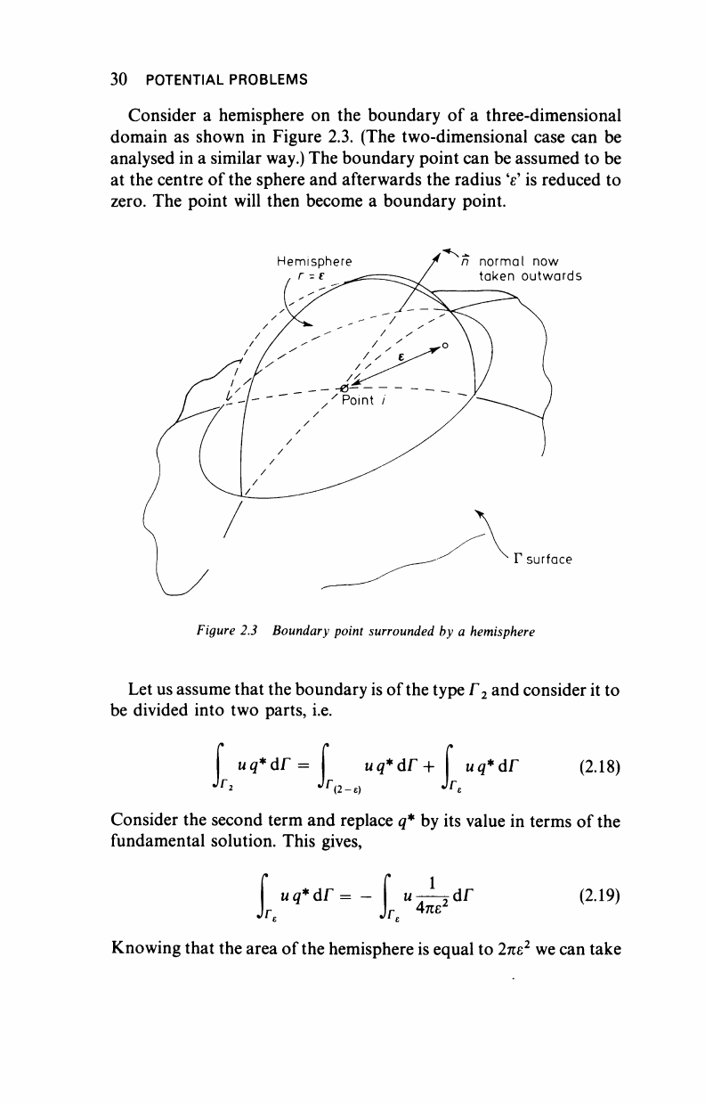
30 POTENTIAL PROBLEMS
Consider a hemisphere on the boundary of a three-dimensional
domain as shown in Figure 2.3. (The two-dimensional case can be
analysed in a similar way.) The boundary point can be assumed to be
at the centre of the sphere and afterwards the radius 'ε' is reduced to
zero.
The point will then become a boundary point.
Hemisphere n normal now
taken outwards
Γ surface
Figure 2.3 Boundary point surrounded by a hemisphere
Let us assume that the boundary is of the type Γ
2
and consider it to
be divided into two parts, i.e.
uq*dr = uq*dr+ uq*dr (2.
18)
Consider the second term and replace q* by its value in terms of the
fundamental solution. This gives,
I
uq*dr =
—
Γ
4πε
2
(2.19)
Knowing that the area of
the
hemisphere is equal to 2πε
2
we can take
POTENTIAL PROBLEMS 31
(2.19) to the limit, i.e. let ε
-►
0 and u-^u
h
which gives
lim f - [ u-^άΓ = lim ( -±u
t
) = -±ii
f
(2.20)
ε-0 Jr
e
4πε
/ «-0
Note that as the ε is now zero the boundary Γ
(2
_
ε)
again can be
represented as Γ
2
and that we have integrated over the singularity,
which gives
—
u
x
. The same result
(
—
u
{
) is obtained in two-
dimensional problems with smooth boundaries.
The right-hand side integrals in equation (2.17) do not give any
singularity. This can be shown by taking the limit of the following
integral when ε
-►
0, i.e.
!™{i«"'
dr
y^{i^
dr
)=°
,22i
>
Substituting the result given by equation (2.20) into our original
relationship (2.17) we obtain the following for a point on the
boundary:
in, + bu*dQ+ uq*dr +
JQ
Jr
2
J
=ί
Ά
""
Γ
Λ
uq*dr
qu*dr+ qu*dr (2.22)
The same result would be obtained if instead of considering the
point on the Γ
2
part of the boundary, we considered it to be on the Γ
part.
Equation (2.22) can be written in a more compact way as follows,
±ιι,+ 6n*dQ+ uq*dr= qu*dr (2.23)
where Γ =
Γ
ί
+Γ
2
and we then apply the boundary conditions u = u
on Fj and q = q on Γ
2
.
..................Content has been hidden....................
You can't read the all page of ebook, please click here login for view all page.