
POTENTIAL PROBLEMS 45
some internal points defined by the finite element mesh shown in
Figure 2.7 is given in Table 2.1.
Table
2.1
COMPARISON
OF
VALUES
OF U FOR SOME
INTERNAL
POINTS
DEFINED
BY FINITE ELEMENT MESH SHOWN IN FIGURE 2.7
Node
Finite
element
Constant
boundary
element
Cell
collocation
16
27
44
46
58
63
1154
0-801
0-404
1-205
1-205
0-768
1-227
0-824
0-426
1-217
1-214
0-776
1-230
0-829
0-416
1-210
1-210
0-771
2.5 POISSON'S EQUATION
In many practical problems we need to introduce body type forces
into the formulation which are acting on the volume or area of the
body but will not add any internal unknowns to the formulation.
The starting expression is given by equation (2.23), i.e.
*i
bu*dQ +
Q
uq*di = qu*
άΓ
(2.68)
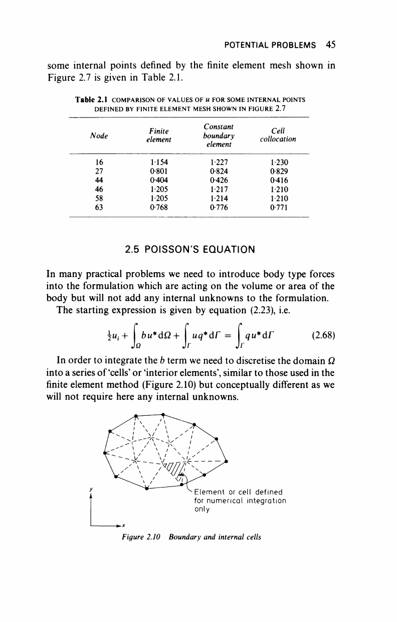
In order to integrate the b term we need to discretise the domain Ω
into a series of'cells' or Interior elements', similar to those used in the
finite element method (Figure 2.10) but conceptually different as we
will not require here any internal unknowns.
Element or cell defined
for numerical integration
only
Figure 2.10 Boundary and internal cells
46 POTENTIAL PROBLEMS
Consider M internal elements, we can then write,
B
t
=
bu*dQ= £ ( bu*dr ) (2.69)
JQ
k
=
1
Jr
k
)
Over each element a numerical integration formula can then be
applied, such as,
bu*dQ= X ( X w
r
(bu*)
r
)A
k
(2.70)
?
k
=
1
r - I /
where r is the integration point, w
r
the weighting function, S the total
number of integration points on each k cell and A
k
the area of the
cell.
Hence for each boundary point
Ί"
equation (2.68) can be written in
discretised form as follows,
B,+
Z
H
u
u
J = Σ Giili (2·
71
)
where the H
0
and G
0
terms are the same as discussed previously
(Section 2.4).
The whole set of equations for the N nodes can be expressed in
matrix form as follows,
B + HU = GQ (2.72)
Note that N
l
values of u and N
2
values of q are known on the
boundary. Hence equations (2.72) are reordered in such a way that all
the unknowns are on the left-hand side. This gives,
AX = F (2.73)
where the F vector contains the terms of B.
Once the values of
u
and q are known over the whole boundary we
can calculate their values at any internal points taking into account
the contribution of the b terms. For instance, the internal value of
u
at
an internal point i is now given by,
"i= Σ
G
ijqj
-
Σ HtjUj-Bi (2.74)
j = i j = i
Similar considerations can be made for the source solution. Here
..................Content has been hidden....................
You can't read the all page of ebook, please click here login for view all page.