
COMBINATION OF REGIONS 181
problems for which approximations could be used to represent the
boundary conditions with good results. As mentioned, the full
potential of these approximations has not yet been fully investigated.
One of the more interesting features of the boundary element
method is the simplicity of the input data required to run a
homogeneous problem. Instead, in finite elements and other domain
methods the amount of data needed is usually very large. This is an
important practical point as many man hours are usually spent in
preparing and checking finite element data.
The accuracy of boundary elements is generally superior to that of
finite elements, except for a narrow boundary layer. Boundary
elements (being mixed type formulation) also produce good results
for the two types of variables under consideration (i.e. potentials and
fluxes or displacements and stresses). The method is better suited to
analyse problems with stress or flux concentrations for which finite
elements is generally unsuited due to the interpolation functions used.
The main disadvantages of boundary elements are the difficulties
encountered in non-homogeneous problems (i.e. finding the fundam-
ental solutions and defining the interfaces) and the fact that all
matrices are now fully populated. In this chapter we will describe how
these disadvantages can be overcome by subdividing the body into
regions. This subdivision is also needed for bodies with different
dimensions in different directions (e.g. slender beams).
7.2 DIVISION INTO REGIONS
In many practical applications it is necessary to divide the body into
several regions. This may be due to having a non-homogeneous body
or because the dimensions of the body are not regular. Long bodies
for instance may produce numerical accuracy problems as the
influence of some nodes over others becomes very weak.
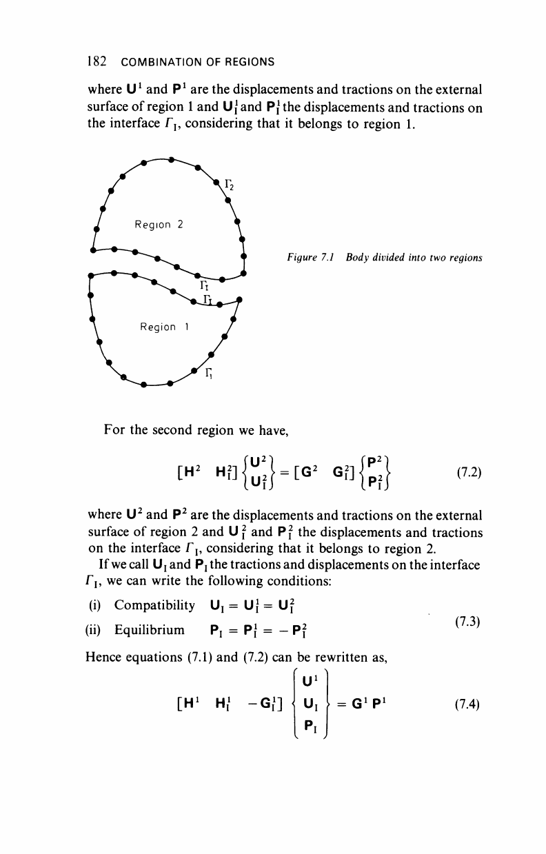
Consider for instance the case of a two-dimensional body for
simplicity divided into two different regions (Figure 7.1). The
interface between the two regions will be called Γ
γ
and two different
fundamental solutions will apply over the parts
1
and 2 of the domain.
Let us analyse the two parts separately. On the first region we have
[H
1
HnjJJ^-Εβ
1
Qajp!}
(7.1)
182 COMBINATION OF REGIONS
where U
1
and P
1
are the displacements and tractions on the external
surface of region
1
and
U{
and Pjthe displacements and tractions on
the interface Γ
Ι?
considering that it belongs to region 1.
Figure 7.1 Body divided into two regions
For the second region we have,
en
(7.2)
where U
2
and P
2
are the displacements and tractions on the external
surface of region 2 and U
2
and
P
f the displacements and tractions
on the interface f,, considering that it belongs to region 2.
If we call Uj and
P!
the tractions and displacements on the interface
Γ,,
we can write the following conditions:
(i) Compatibility U, = U} = U
2
(ii) Equilibrium P, = P} = - P
2
Hence equations (7.1) and (7.2) can be rewritten as,
U
1
[H
1
Hi -Gi] V
}
1 = G'P
1
Pi
(7.3)
(7.4)
COMBINATION OF REGIONS 183
[H
2
Hf Gf]
U
2
U,
^
= G
2
P
2
D
2
Equations (7.4) and (7.5) can be written together as follows,
,'Uf
H
1
|Hf -G}
G?
0
H
2
interface
u,
Pi
U
2
>
=
G
1
0
0 G
2
(7.5)
(7.6)
The system needs still to be recorded according to the prescribed
displacements and tractions.
This solution has the added advantage that the system of equations
is now banded. Note that compatibility and equilibrium are explicitly
satisfied between regions (in
finite
elements instead only compatibility
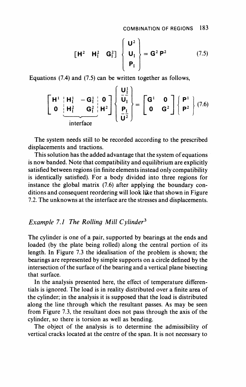
is identically satisfied). For a body divided into three regions for
instance the global matrix (7.6) after applying the boundary con-
ditions and consequent reordering will look like that shown in Figure
7.2.
The unknowns at the interface are the stresses and displacements.
Example 7.1 The Rolling Mill Cylinder*
The cylinder is one of a pair, supported by bearings at the ends and
loaded (by the plate being rolled) along the central portion of its
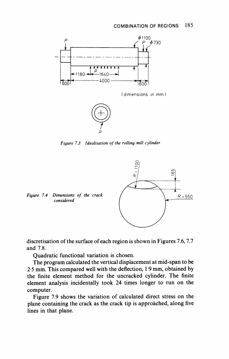
length. In Figure 7.3 the idealisation of the problem is shown; the
bearings are represented by simple supports on a circle defined by the
intersection of the surface of the bearing and a vertical plane bisecting
that surface.
In the analysis presented here, the effect of temperature differen-
tials is ignored. The load is in reality distributed over a finite area of
the cylinder; in the analysis it is supposed that the load is distributed
along the line through which the resultant passes. As may be seen
from Figure 7.3, the resultant does not pass through the axis of the
cylinder, so there is torsion as well as bending.
The object of the analysis is to determine the admissibility of
vertical cracks located at the centre of the span. It is not necessary to
184 COMBINATION OF REGIONS
Unknowns Unknowns Unknowns Unknowns Unknowns
on on on on on
Γι interface Γ
12
Γ
2
interface Γ
23
Γ
3
Equations
for
region 1
Equations
for
region 2
Equations
for
region 3
Figure 7.2 Banded matrix equations
corresponding
to a body divided into three regions
withdraw a cylinder from service immediately a crack appears; but if
the cylinder fails whilst in operation, considerable damage is done to
other components such as the bearings. For the purposes of analysis,
the crack tip is supposed to be circular (Figure 7.4).
The modulus of elasticity was taken to be 210000 N mm"
2
and
Poisson's ratio 0-3. The intensity of
the
line load was nearly constant,
8500 N mm
-1
, and the length of the perpendicular from the axis of
the
cylinder to the resultant was 40
mm.
There was therefore very little
torsion and the critical case may be taken to be that in which the crack
is diametrically opposed to the load point. The crack considered here
was of depth 165 mm and radius
1100
mm.
The cylinder was divided
into 5 regions (Figure 7.5), the fifth containing the crack. The
COMBINATION OF REGIONS 185
600
#1100
/ P ΦΊ30
-1180^-U—1640-
-4000-
K
I600I
( dimensions in mm )
Figure 7.3 Idealisation of
the
rolling mill cylinder
Figure 7.4 Dimensions of the crack
considered
discretisation of the surface of each region is shown in Figures
7.6,7.7
and 7.8.
Quadratic functional variation is chosen.
The program calculated the vertical displacement at mid-span to be
2-5 mm. This compared well with the deflection, 1-9 mm, obtained by
the finite element method for the uncracked cylinder. The finite
element analysis incidentally took 24 times longer to run on the
computer.
Figure 7.9 shows the variation of calculated direct stress on the
plane containing the crack as the crack tip is approached, along five
lines in that plane.
..................Content has been hidden....................
You can't read the all page of ebook, please click here login for view all page.