
ELASTOSTATICS 133
movements. Let us assume we have a unit rigid body displacement in
any one direction; equation (5.46) then becomes,
ΗΙ,
= 0 (5.48)
where l
z
is a vector defining a unit rigid displacement in the direction
T. Hence the diagonal terms of
H
are simply
(5.49)
which means that the c coefficients do not need to be determined
explicitly.
Once equations (5.47) have been solved we know the stresses and
displacements over the whole surface of the body. We can now
compute the stresses and displacements at any internal point.
STRESSES AND DISPLACEMENTS INSIDE THE BODY
The displacements at any point inside the body are given by equation
(5.28),
i.e.
u*bdi2
(5.50)
u =
u*pdr-
p*udr
+
or for each / component at that point,
"i= I u?
kPk
dr- I
P
r
k
u
k
dr+ I uf
k
b
k
dQ (5.51)
Jr Jr JQ
The internal stresses for an isotropic medium can be obtained by
applying equation (5.8)
. - du
t
fdUi du:
Substituting (5.51) into (5.52) we obtain,
(5.52)
P
k
dr-
u
k
dr
+
(5.53)
134 ELASTOSTATICS
We can write this as
σ„ = ί D
kij
p
k
dr-[ S
kij
u
k
dr+ D
kij
b
k
άΩ (5.54)
Jr Jr h
'kijPkdi
where for three dimensions,
dr dr dr Ί 1
δχι dxj dx
k
J 8π(1
—
v)
Ί[«-*<
+
·(^
+ί
.£)-
dr dr dr Ί / dr dr dr
dx
t
dxj dx
k
J
'
dxj dx
k
J
dx
t
+ 3
2μ
(5.55)
S
"
J
~ 3r
dr_
dx
t
.,-.,„ dr dr · ~ .
+ (1 - 2v)
3
n
k
— — +
n,
S
ik
+
n,S
Jk
-
■{l-4v)n
k
S,j
dxi dxj
1
8«(l-v)
(5.56)
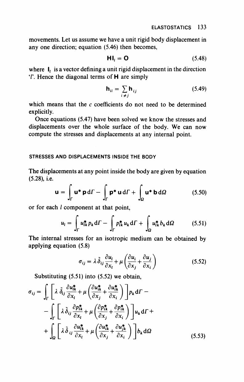
The derivatives of r with respect to the coordinates are shown in
Figure 5.4 for a two-dimensional case for simplicity.
Boundary point
M. . xf-rf
Figure 5.4 Derivatives ofr: P, interior
point;
B, boundary point
ELASTOSTATICS 135
Example 5.1
1
As
an example of the application of the above techniques, consider the
problem of determining
the
stress concentration for
a
spherical cavity.
Cruse used an equation similar to (5.27) as the starting point of his
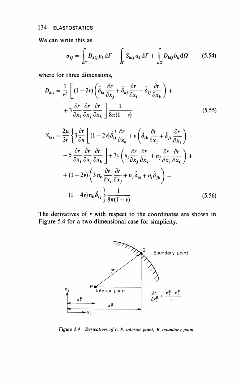
analysis. Then discretising the surface of the problem region (Figure
5.5) he
was
able to represent the region using quadratic curved surface
elements. (The triangular elements shown in Figure 5.5 are just
degenerate elements with essentially the same form.) To represent the
surface curvature Cruse used quadratic shape functions to map
the elements and as he used quadratic interpolation functions on
each element his formulation was of the isoparametric form, (see
Chapter 3.)
w
=
5'
σ
=
10,000 psi
E= 18 x 10
6
psi
ν
=
0·3
Figure 5.5 Boundary element discretisation for spherical cavity 6 elements
(cylinder 2, cavity 4), 28 nodes
136 ELASTOSTATICS
By exploiting the symmetry of the problem he was able to represent
the surface using only six elements.
2-5
NcT
2-0
E=
18
x
10
b
psi
=
0-3
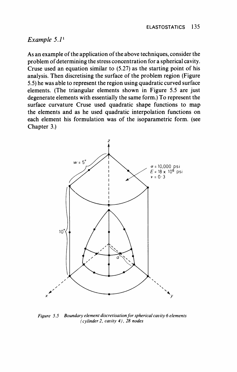
Figure 5.6 Stress concentration for a spherical cavity. K
TN
—
a
m
Ja where σ - σ/[1
-
(ö/w)
2
];
the full curve is from Peterson and the data points are from boundary integral
equations: O, quadratic; V, linear
The results for the stress concentration shown in Figure 5.6 show
good agreement with published results and also compare the results
using the quadratic isoparametric boundary elements, with the
corresponding results obtained using the simpler linear boundary
elements.
Example 5.2
1
In the same paper referred to above, Cruse has studied the problem of
crack propagation by looking at the stresses around a circular crack,
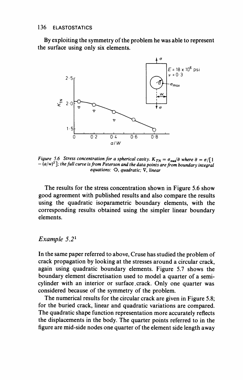
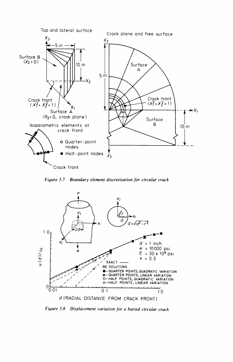
again using quadratic boundary elements. Figure 5.7 shows the
boundary element discretisation used to model a quarter of a semi-
cylinder with an interior or surface.crack. Only one quarter was
considered because of the symmetry of the problem.
The numerical results for the circular crack are given in Figure 5.8;
for the buried crack, linear and quadratic variations are compared.
The quadratic shape function representation more accurately reflects
the displacements in the body. The quarter points referred to in the
figure are mid-side nodes one quarter of
the
element side length away
Top and lateral surface
-5 in —
Surface B
(X
2
=
0)
Crack front
(Xf+X
2
2
=),
i x
Surface A
(X
3
=0,
crack plane)
Isoparametric elements at
crack front
Crack plane and free surface
Xi
5 in
o Quarter-point-
nodes
• Half-point nodes ^
Crack front
Figure 5.7 Boundary element discretisation for circular crack
d^iä^P-
d - 1 inch
σ = 10000 psi
E = 30 x 10
6
psi
v = 0 3
EXACT
BE SOLUTIONS
■ -QUARTER
POINTS,
QUADRATIC VARIATION
A-QUARTER POINTS, LINEAR VARIATION
□-HALF
POINTS, QUADRATIC VARIATION
Δ-HALF POINTS, LINEAR VARIATION
0-01 01 10
a
7
(RADIAL DISTANCE FROM CRACK FRONT)
Figure 5.8 Displacement variation for a buried circular crack
..................Content has been hidden....................
You can't read the all page of ebook, please click here login for view all page.