
102 FUNDAMENTAL SOLUTIONS
+ 3
12
(b)
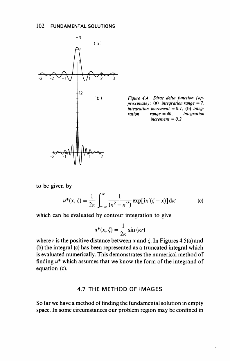
Figure 4.4 Dirac delta function (ap-
proximate)
:
(a) integration range = 7,
integration increment =0.1; (b) integ-
ration range = 40, integration
increment = 0.2
(c)
to be given by
Β
*
(χ
·
ο=
έΓ-ί?^)
βχρ[ίκ
'
ίί
"
χ)]ακ
'
which can be evaluated by contour integration to give
u*(x, ζ) = --sin (ΚΓ)
2K
where r is the positive distance between x and ξ. In Figures 4.5(a) and
(b) the integral (c) has been represented as a truncated integral which
is evaluated numerically. This demonstrates the numerical method of
finding u* which assumes that we know the form of the integrand of
equation (c).
4.7 THE METHOD OF IMAGES
So far we have a method of finding the fundamental solution in empty
space. In some circumstances our problem region may be confined in

FUNDAMENTAL SOLUTIONS 103
Figure 4.5 Approximate fundamental solution for the one-dimensional Helmholtz
equation, κ = 1.1: (a) integration range = 5, integration increment = 0.2;
(b) integration range = 20, integration increment = 0.2
some regular way and it may be more convenient to find a
fundamental solution specific to a region.
The simplest case is that of
a
semi-infinite space such as may occur
in a foundation or fluids problem. The surface of the soil or fluid may
make it more convenient to work with a semi-infinite space funda-
mental solution. We choose this solution to satisfy the boundary
condition on the interface identically; in this way we shall not need to
put elements on the surface when using the boundary integral
method.
To obtain these solutions it is necessary to consider their physical
interpretation. Consider for the moment a two-dimensional space
and take coordinates as in Figure 4.6. The interface is along the x
l
axis
and the normal to this is measured in the positive x
2
direction. We
shall require that du/δη = 0 on this interface.
The fundamental solution is the field due to a point source in
infinite space and so the field in the presence of our boundary x
2
= 0
will represent our half space fundamental solution. Consider a source
strength m at a point (ξ
ί9
—a).
104 FUNDAMENTAL SOLUTIONS
*2
Image strength m'
j
n
Interface
du
dn
=
0
Observation point
"* Source strength m
(ί,-α)
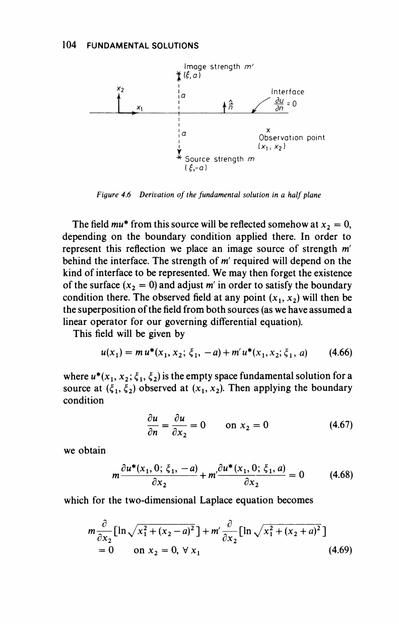
Figure 4.6 Derivation of
the
fundamental solution in a half
plane
The field
mw*
from this source will be reflected somehow at x
2
= 0,
depending on the boundary condition applied there. In order to
represent this reflection we place an image source of strength m'
behind the interface. The strength of
m!
required will depend on the
kind of interface to be represented. We may then forget the existence
of the surface (x
2
= 0) and adjust
m'
in order to satisfy the boundary
condition there. The observed field at any point (x
l9
x
2
) will then be
the superposition of the
field
from both sources (as we have assumed a
linear operator for our governing differential equation).
This field will be given by
w(x
1
) = mw*(x
1
,x
2
; ξ
ΐ9
-a) + m'u*(x
u
x
2
'^
u
a) (4.66)
where
u*(x
l9
x
2
; ξ
ΐ9
ζ
2
) is the empty space fundamental solution for a
source at (ξ
ΐ9
ξ
2
) observed at (x
1?
x
2
). Then applying the boundary
condition
du du
^- = τ— = 0 οηχ
2
= 0
en cx
2
(4.67)
we obtain
m
du*(
Xl
,0^
u
-a)
+ m
,^*(*i,0;^a)
= Q (4 6g)
dx
7
dx
0
which for the two-dimensional Laplace equation becomes
m —
[In
Jx + (x
2
-a)
2
] +
™'
—
[In
Jx + (x
2
+ 0)
2
]
= 0 on x
2
= 0,
V
x
x
(4.69)
FUNDAMENTAL SOLUTIONS 105
or in particular at x
x
=0 gives
-^- + *-0 (4.70)
— a a
Hence we choose m' = m. The field is then
u = ^ jln U/x
2
+ (x
2
-a)
T
] +
In
[Jx + (x
2
+
«)
T
~]
j (4.71)
= ^ln|
x
/[x? + (x
2
-«)
2
][xi + (x
2
+ a)
2
]J (4.72)
Thus the fundamental solution for the two-dimensional Laplace
equation for the lower half plane is (Figure 4.6)
κ*(χ,, x
2
; ξ
ι
,ξ
2
) = —In i ^/[(x, -ξ
χ
)
2
+ (χ
2
-ξ
2
ψ~~
χ
Note. We have that wf is the solution of
M
* = mö(x
u
x
2
— a)
+ mö(x
u
x
2
+
a)
(4.74)
t
. t
source image
We could equally have solved this equation in the usual way.
For different boundary conditions we obtain a slightly different
equation for m, i.e. if u = 0 on x
2
= 0 then m = m' and
,1/2
u
*
=
h
ln
Yxf +
fa-^Y
/a
1
(475)
in this case.
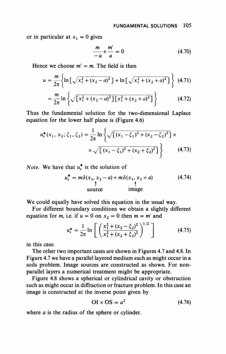
The other two important cases are shown in Figures 4.7 and 4.8. In
Figure 4.7 we have a parallel layered medium such as might occur in a
soils problem. Image sources are constructed as shown. For non-
parallel layers a numerical treatment might be appropriate.
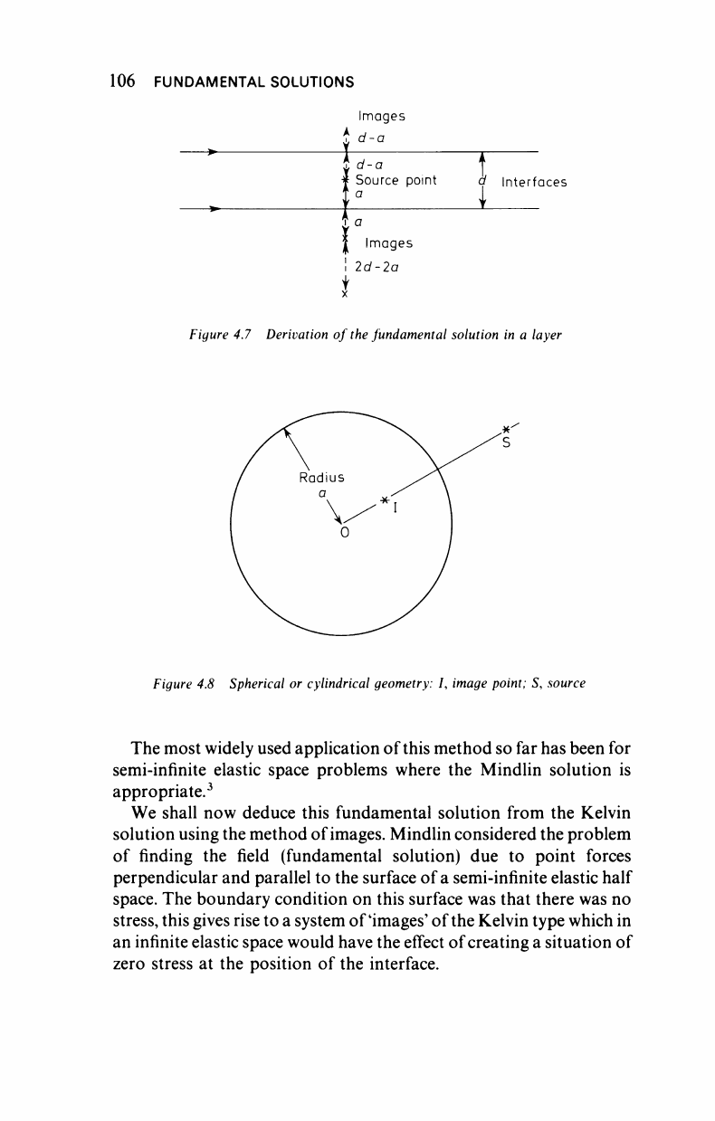
Figure 4.8 shows a spherical or cylindrical cavity or obstruction
such as might occur in diffraction or fracture problem. In this case an
image is constructed at the inverse point given by
OI x OS = a
2
(4.76)
where a is the radius of the sphere or cylinder.
106 FUNDAMENTAL SOLUTIONS
Images
ί
d-a f
* Source point d Interfaces
J Images
! 2d-2a
i
Figure 4.7 Derivation of
the
fundamental solution in a layer
Figure 4.8 Spherical or cylindrical geometry: I, image point; S, source
The most widely used application of this method so far has been for
semi-infinite elastic space problems where the Mindlin solution is
appropriate.
3
We shall now deduce this fundamental solution from the Kelvin
solution using the method of images. Mindlin considered the problem
of finding the field (fundamental solution) due to point forces
perpendicular and parallel to the surface of a semi-infinite elastic half
space. The boundary condition on this surface was that there was no
stress,
this gives rise to a system of'images' of the Kelvin type which in
an infinite elastic space would have the effect of creating a situation of
zero stress at the position of the interface.
..................Content has been hidden....................
You can't read the all page of ebook, please click here login for view all page.