
POTENTIAL PROBLEMS 47
we start with equations (2.35) and (2.36) including boundary terms, i.e.
bu*dQ
u
t
= σιι*άΓ
—
Jr
J
(k
_ _1
I^ +
aq*dr-
bq*dQ
and integrate them numerically, which gives,
j= i
J=l
(2.75)
(2.76)
The terms 5" and Β
ρ
can be obtained applying numerical integration.
Once the boundary conditions are applied, the system of equations
(2.76) can be written in the same form as (2.73).
2.6 THE ORTHOTROPIC CASE
In many engineering applications the material properties cannot be
considered to be isotropic and we need to consider them as
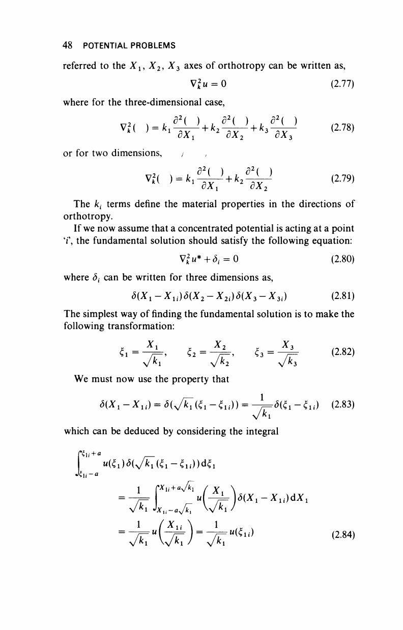
orthotropic. Let us study the case of a body such as the one
represented in Figure 2.11. The governing equation for this system,
X
}
Y
direction of
orthotropy
Figure 2.11 Orthotropic medium
48 POTENTIAL PROBLEMS
referred to the
X
l9
X
2
,
X
3
axes of orthotropy can be written as,
V£u
=
0 (2.77)
where for the three-dimensional case,
Vl(
)
= ki
^x7
+k
>-M7
+k
>^x7
(178)
or for two dimensions,
j
d
2
(
) d
2
( )
v
<
(
) =
fcl
^V
+
*
2
^7
(179)
The
k
t
terms define the material properties in the directions of
orthotropy.
If
we
now assume that a concentrated potential is acting at a point
T, the fundamental solution should satisfy the following equation:
V
k
2
w*-h^
=
0 (2.80)
where S
t
can be written for three dimensions as,
δ(Χ
ι
-Χ
ίί
)δ(Χ
2
-Χ
2ί
)δ(Χ,-Χ
3ί
)
(2.81)
The simplest way of finding the fundamental solution is to make the
following transformation:
We must now use the property that
^i-^ii) = iU/Mii -in)) = -4=5«!-«!,) (2.83)
V
fc
i
which can be deduced by considering the integral
"«iWVfcliil-ili))^!
1 f*i; + <Ai
/
Y
-
= ηΙ-
7
^δ(Χ
ι
-Χ
ιί
)άΧ
1
U
(4^)
=
^"
(ili)
(2-84)
^1
v
^1
/ V^l
POTENTIAL PROBLEMS
49
where a is a positive constant. Hence equation (2.80) can be written
(Pu fru_ dht_ 1_
= 0 (2.85)
v2
"
= ^+-Ü2 + ^+ /r-r-^i-^fo-^Ka-fr,)
The fundamental solution of equation (2.85) is as previously
1 1
(2.86)
4πΓ
0
JkJ,k
3
where,
r
0
= V«+
«!
+ Ǥ = ^ff + ff + ff (2.87)
The same transformation applied
to
two-dimensional problems
produces,
w*
=
*=ln
(
~ |
(2.88)
where
now
-
M
FLUX
AT
THE BOUNDARY
Consider
the
two-dimensional case
for
simplicity.
In
order
to
calculate
the
flux
at the
boundary
we can
apply Green's theorem,
which gives,
Ω
fc
1^2+
fc
2 7^2 )
αΩ
=
kl
^
nX
+
kl
l^
nY
^
(289)
where
n
x
=
cos
(M,
X),
M
y
=
cos
(n,
Γ)
The term between brackets
in the
right-hand side
is the
internal flux
..................Content has been hidden....................
You can't read the all page of ebook, please click here login for view all page.