
HIGHER-ORDER ELEMENTS 55
3.2 LINEAR ELEMENTS FOR TWO-DIMENSIONAL
PROBLEMS
Let us consider here a linear variation for u and q for which case the
nodes are now considered to be at the intersection between two
straight elements such as those shown in Figure 2.4(b).
Equation (2.42) can now be written,
CtUi-l·
Σ f uq*dr= Σ f qu*dr (3.1)
j = i Jr, j = i Jr,
Note that the - coefficient of u
t
has been replaced
by
an unknown
c
f
value. This is because c, is equal to
—
only for a smooth boundary.
The determination of
c,
is rather complex but it will soon be shown
that it does not need to be known explicitly and this simplifies the
formulation.
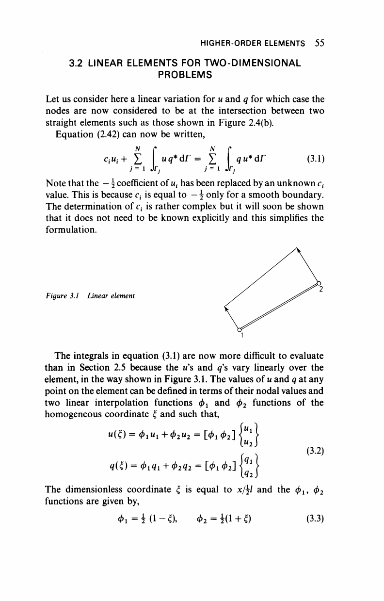
Figure 3.1 Linear element
The integrals in equation (3.1) are now more difficult to evaluate
than in Section 2.5 because the w's and g's vary linearly over the
element, in the way shown in Figure
3.1.
The values of
u
and
q
at any
point on the element can be defined in terms of their nodal values and
two linear interpolation functions φ
ί
and φ
2
functions of the
homogeneous coordinate ξ and such that,
*(ξ) = *i«i +<M
2
= [0i Φι]
j"
1
|
(3.2)
qtt) = <Mi +
0
2
42
= ίΦι Φι]^
1
The dimensionless coordinate ξ is equal to x/jl and the φ
ί
, φ
2
functions are given by,
Φι=±(1-& *2=i(l + ö (33)
56 HIGHER-ORDER ELEMENTS
The integrals along a segment; on the right-hand side of equation
(3.1) can be written as,
(3.4)
where
h}
}
=
<t>
iq
*dr, hfj=
f
<i>
2
q*ar
Jrj Jr,
The h^j are influence coefficients defining the interaction between
the point 'f under consideration and a particular
k
node on an element
For the integrals on the right-hand side of (3.1) we can write,
[
qu*dr=
f
[^^
2
]«*dr|^
-lehetjl
(3.5)
with,
βΐ-
>άΓ
|
φ^+άΓ,
gfj= </>
2
w*<
»o
Jo
To write the equation corresponding to node T in discrete form we
need to add the contribution from two adjoining elements, (j
—
1)
and
(;), into one term, defining the nodal coefficient. This will give the
following equation:
u~>
I q
2
c
i
u
i
+ [H
il
H
i2
...H
iN
]{
= [GiiG«...G
w
K
{«N)
M3-6)
where each H
i}
term is equal to the h
2
term of element 'j - Γ plus the
h
1
term of element (j
—
1) for a clockwise numbering system. The
same applies for G
0
. Hence formula (3.6) represents the assembled

HIGHER-ORDER ELEMENTS 57
equation for node T and it can be written as,
c
iUi
+ Σ #0";= Σ
G
u
qj
(3.7)
j = i 7 = i
or more simply,
Σ "o";= Σ ^υ·^· (3.8)
7=1 7=1
where
Hij^Hij
for i#7
Hij = Hij +
Ci
for 1=7
When all the nodes are taken into consideration, equation (3.8)
produces an
JV
x iV system of equations which can be represented in
matrix form as follows,
HU = GQ (3.9)
If
the
surface is not smooth at the point T the c
{
=
— ^
is no longer
valid but one can calculate the diagonal terms of H by using the fact
that when a uniform potential is applied on the whole boundary the
values of q's must be zero. Under this condition equation (3.9)
produces,
H I = 0 (3.10)
Equation (3.10) indicates that the sum of
all
the elements of
H
in a
row ought to be zero, hence the values of the coefficients in the
diagonal can be easily calculated once the off-diagonal coefficients are
all known, i.e.
H
u
=-
£ tf
u
(3.11)
Example 3.1
The Saint Venant torsion of a prismatic beam is governed by a
differential equation of the type
d ( du d ( du
58 HIGHER-ORDER ELEMENTS
where G is the shear modulus and
Θ
is the rate of twist. The problem
variable is the stress function u, such that
X
" =
W
hz=
~^c
(b)
T'S
are the shear stresses, u must have a constant value on the
boundary. For convenience it is normally assumed that such constant
is equal to zero. Considering an homogeneous material we can write,
dx
2 +
dy
2
^ϊ + ^2=
2
(c)
where v = u/G6.
This problem can be solved for v, but noticing that the rate of twist
Θ
is so far unknown. We know that the torque M
t
is
M
t
= JG0 = 2 udxdy (d)
where J is the torsional rigidity. We can therefore compute J by
evaluating the following integral:
J = 2 v dxdy (e)
The rate of twist is then given by
Θ
= MJGJ (f)
Finally we can compute the shear stresses as
dv
r
- re
dv
τ
χζ =
0Θ
77'
x
y* = ~
G0
7Γ (8)
Consider as an illustration the problem of the torsion of a prismatic
bar of elliptical cross section, defined by the equation,
x
2
y
2
a b
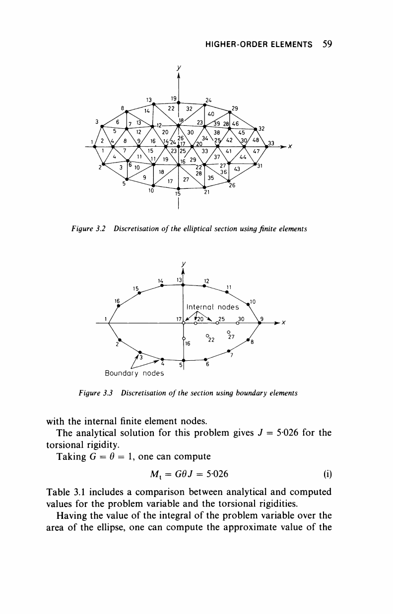
For this example we take a = 2 and b = 1. A finite element mesh
selected, consisting of 33 nodes and 48 linear elements is shown in
Figure 3.2.
The same example was solved using linear boundary elements
(Figure 3.3) with 16 nodes and a series of internal points coinciding
HIGHER-ORDER ELEMENTS 59
Figure 3.2 Discretisation of the elliptical section using finite elements
* 5
Boundary nodes
Figure 3.3 Discretisation of
the
section using boundary elements
with the internal finite element nodes.
The analytical solution for this problem gives J = 5Ό26 for the
torsional rigidity.
Taking G =
Θ
= 1, one can compute
M
t
= G6J = 5026
(i)
Table 3.1 includes a comparison between analytical and computed
values for the problem variable and the torsional rigidities.
Having the value of the integral of the problem variable over the
area of the ellipse, one can compute the approximate value of the
..................Content has been hidden....................
You can't read the all page of ebook, please click here login for view all page.