
TIME-DEPENDENT AND NON-LINEAR PROBLEMS 169
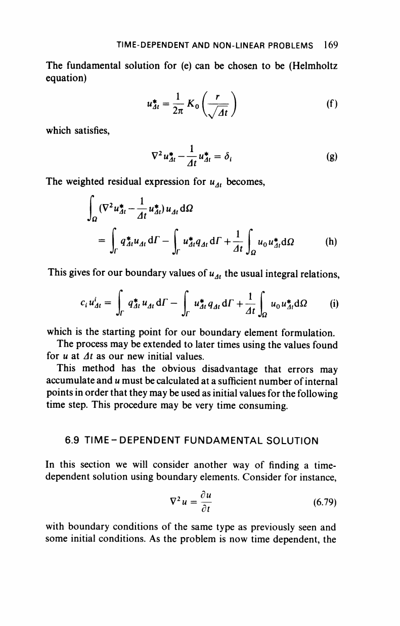
The fundamental solution for (e) can be chosen to be (Helmholtz
equation)
"
3
'4
K
°fe)
which satisfies,
(f)
ν
2
«5,-^«5,
= *
(
(g)
The weighted residual expression for u
At
becomes,
i
^
2
<-j
t
^
t
)u
at
dQ
= 1 i*^i
dr
-
u%q
At
dr
+ — u
0
u*
t
dQ (h)
This gives for our boundary values of u
At
the usual integral relations,
Ci*4= tät
u
M&
r
-
w
*i^dr+— u
0
u%dQ (i)
Jr Jr Δί]
Ω
which is the starting point for our boundary element formulation.
The process may be extended to later times using the values found
for u at At as our new initial values.
This method has the obvious disadvantage that errors may
accumulate and
u
must be calculated at a sufficient number of internal
points in order that they may be used as initial values for the following
time step. This procedure may be very time consuming.
6.9 TIME-DEPENDENT FUNDAMENTAL SOLUTION
In this section we will consider another way of finding a time-
dependent solution using boundary elements. Consider for instance,
V
2
u = ^ (6.79)
ct
with boundary conditions of the same type as previously seen and
some initial conditions. As the problem is now time dependent, the
170 TIME-DEPENDENT AND NON-LINEAR PROBLEMS
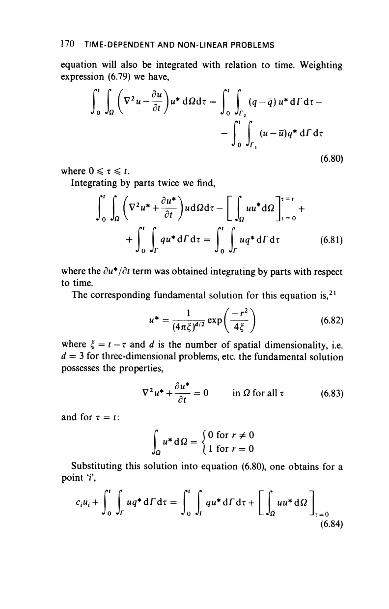
equation will also be integrated with relation to time. Weighting
expression (6.79) we have,
Π
V
2
u--^-
]u*dOdi
=
f f
(q-q)u
Jo Jr
2
(u-ü)q*
o Jr,
♦dfdi-
άΓάτ
(6.80)
where 0 < τ ^ ί.
Integrating by parts twice we find,
+ qu*drdT= uq*drdz
Jo Jr Jo Jr
+
(6.81)
where the du*/dt term was obtained integrating by parts with respect
to time.
The corresponding fundamental solution for this equation is,
21
~2"
1
(4πξ)<
412
exp
4£
(6.82)
where ξ = t
— τ
and d is the number of spatial dimensionality, i.e.
d = 3 for three-dimensional problems, etc. the fundamental solution
possesses the properties,
V>«* + ^ = 0
dt
in Ω for all τ
(6.83)
and for τ = t:
["•"H
0 for r Φ 0
1 for r = 0
Substituting this solution into equation (6.80), one obtains for a
point V,
Λί Λ C* C [~ Γ ~l
,«,+ Wi?*drdT= 4M*dFdT+ uu*di2
Jo Jr Jo Jr LJß
J
T
= o
(6.84)
TIME-DEPENDENT AND NON-LINEAR PROBLEMS 171
The last term in the above formula corresponds to the initial
conditions at τ = 0. Since the fundamental solution itself is time
dependent, one does not need to propose an iterative scheme to solve
time-dependent problems as it is usually done in finite elements or
finite differences.
When the surface is not smooth at the point T, one can still
calculate the diagonal terms of H by the application of a uniform
potential over the whole domain, which will give zero normal fluxes at
the boundaries. Notice, however, that now equation (6.84) can be
written as,
HU = GQ + P (6.85)
where the vector P depends on the potentials. Thus the coefficients on
the diagonal of H will be given by,
H»= - Σ
H
u +
p
i (6.86)
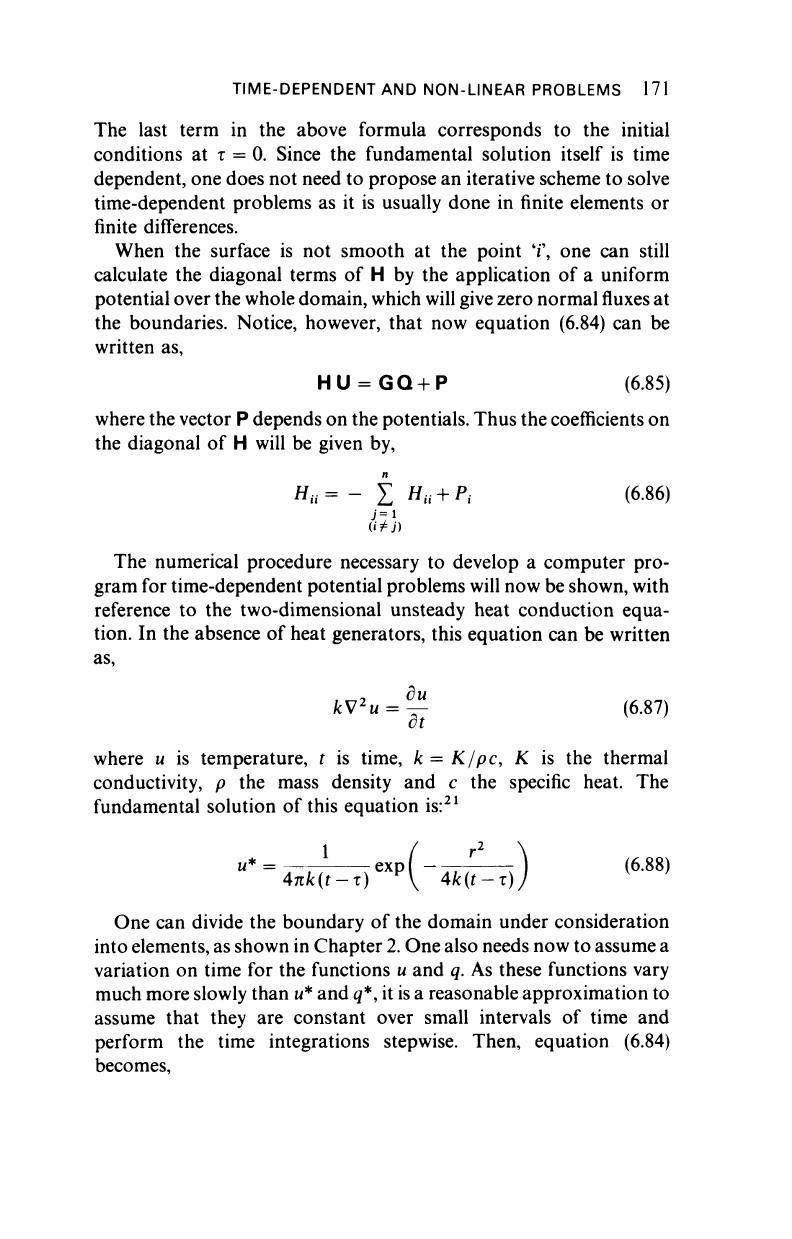
The numerical procedure necessary to develop a computer pro-
gram for time-dependent potential problems will now be shown, with
reference to the two-dimensional unsteady heat conduction equa-
tion. In the absence of heat generators, this equation can be written
as,
fcV
2
w = ^ (6.87)
where u is temperature, t is time, k = K/pc, K is the thermal
conductivity, p the mass density and c the specific heat. The
fundamental solution of this equation is:
21
M
* = TTFi ϊ
ex
P ( " ΎΓ^—Λ )
(
6
·
88
>
4nk(t-x) 4k(t-r)J
One can divide the boundary of the domain under consideration
into elements, as shown in Chapter
2.
One also needs now to assume a
variation on time for the functions u and q. As these functions vary
much more slowly than u* and q*, it is a reasonable approximation to
assume that they are constant over small intervals of time and
perform the time integrations stepwise. Then, equation (6.84)
becomes,
172 TIME-DEPENDENT AND NON-LINEAR PROBLEMS
CfMi
+
k
" q*drdr = k q w*didr +
[Jr*
do
L,
+
| I
MM*
dß I
(6.89)
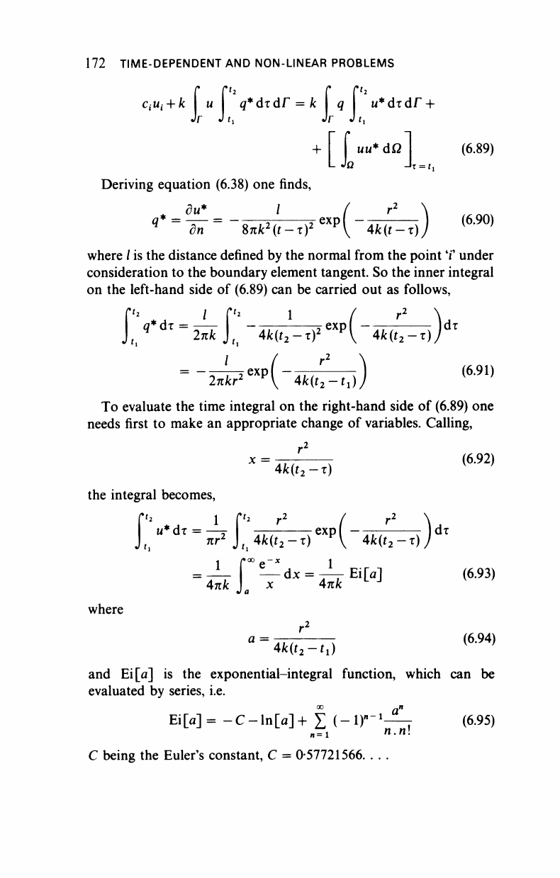
Deriving equation (6.38) one finds,
du*
I ( r
2
q
*
-
^Γ =
-%nkHt-rf^-m^))
(690)
where / is the distance defined by the normal from the point
Ί"
under
consideration to the boundary element tangent. So the inner integral
on the left-hand side of (6.89) can be carried out as follows,
=
-u?
exp
{-4k£^)
(69i)
To evaluate the time integral on the right-hand side of (6.89) one
needs first to make an appropriate change of variables. Calling,
x
=
JUT.
7 <
6
·
92
)
4&(ί
2
-τ)
the integral becomes,
1 Γ°°β"
χ
1
= JL _dx = — Ei|>] (6.93)
Ank )
a
x Auk
where
and Ei[a] is the exponential-integral function, which can be
evaluated by series, i.e.
Ei[a]= -C-ln|>]+ £
(-iy*-^
(6.95)
C being the Euler's constant, C = 0-57721566
..................Content has been hidden....................
You can't read the all page of ebook, please click here login for view all page.