
ELASTOST ATI CS 141
5.6 TWO-DIMENSIONAL ELASTICITY
Let us now apply the boundary element method in two-dimensional
elasticity. The fundamental solution of the governing equations, i.e.
is as following (plane strain)
(5.57)
"Ä
=
Pik =
8πμ(1
4π(1
ι
—-(
— v)r \_dn
{
l-2v)3,
k
+
2^)
+
cx
k
ox^
(5.58)
,1 ,J
dr 8r
+ (l-2v —n
k
- —n,
cx
l
cx
k
where p
lk
and u
lk
represent the tractions and displacements in the k
direction due to a unit force in the / direction.
The elements of p* and u* can be written in matrix form as
follows,
=
ΓΡΤΙ Pia
LP21 P22
ir =
u*
2
«21 "22.
(5.59)
The displacements, tractions and body force vectors are now
u =
P =
b =
(5.60)
The starting equation can be written in matrix form as for three-
dimensional elasticity (equation (5.37)), i.e.
CiUi +
p*udf
=
u*pdr+
u
T Jr JQ
(5.61)
The rest of the matrix operations are similar to those described in
Section 5.5 for the three-dimensional case, but here the boundary
integrals are line integrals and the body force terms are obtained by
integrating over area instead of volume of internal elements.
Once the unknowns are known over all the surface one can find the
142 ELASTOSTATICS
internal displacements and stresses at any internal point using,
i*pdr-
p*udr +
u*bdO
u
-I
u
*ij= DkijPkdr- S
kij
u
k
dr+ D
kij
u
k
dQ
(5
Jr
Jr JQ
(5.62)
63)
where,
$kij —
1
Γ
. Ji 3r
?
dr
?
dr
dr
dr dr Ί 1
+ 2
dx
t
dXj
dx
k
J 4π(1
—
v)
A* L<3r Γ
· 5r Λ 3r
?
or
7
|2-[(l-2vR,.-
+
v^,-
+
^,-
5r
dr dr ~| / dr dr dr
dx
t
dXj
dx
k
J
' dXj
dx
k
j
dx,
+
(5.64)
dr_
dx
k
+ (l-2v)(2n
k
^^ + n
j
ö
ik
+ n
i
ö
jk
) -
-(l-4v)n
k
<5
0
-
1
4π(1-ν)
(5.65)
As previously the integrals can
be
calculated using numerical
integration formulae, or analytically for very simple cases.
Note that in order to pass from plane strain to two-dimensional
plane stress analysis one has to substitute the values of Poisson's ratio
and modulus of elasticity by,
E*>E[
1
(1+v)
2
The thermal strain coefficient is now
1+v
a
4=>
a
;
v<=>
v/(l + v)
(5.66)
l+2v
Example
5A
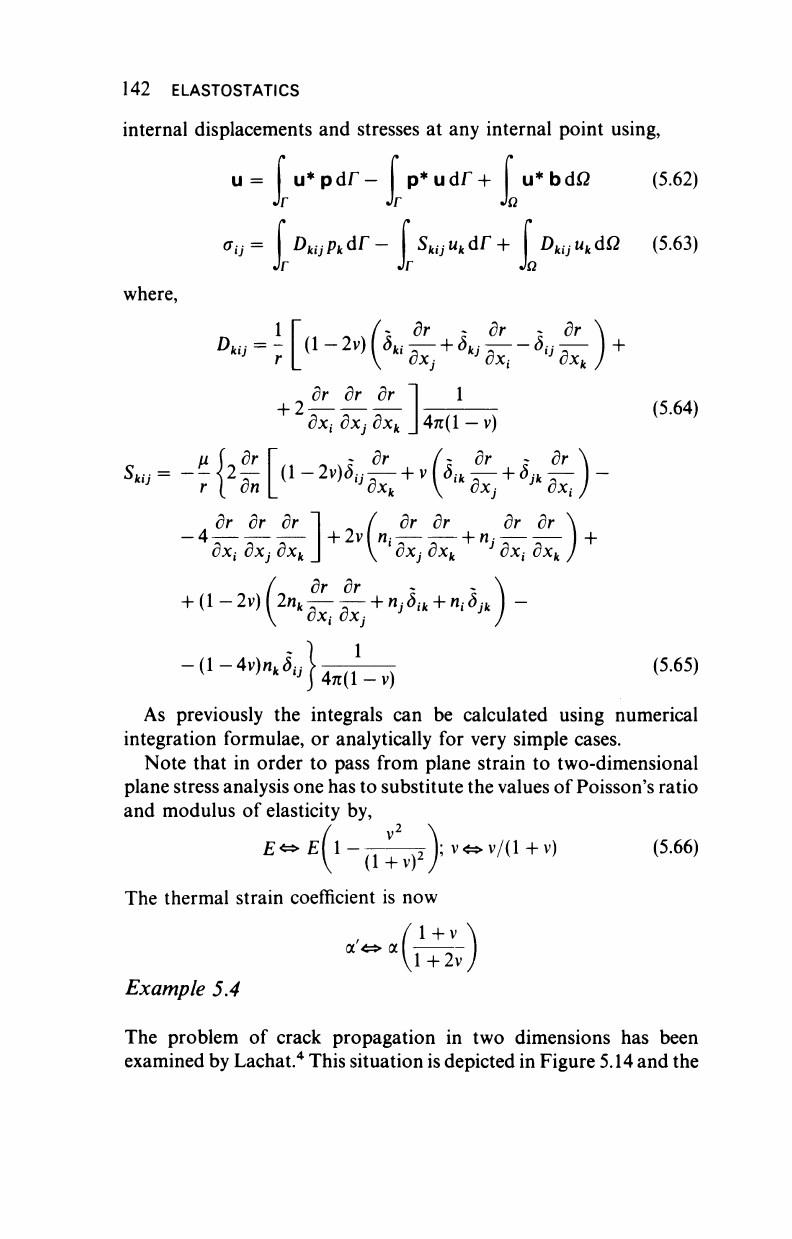
The problem
of
crack propagation
in
two dimensions has been
examined by Lachat.
4
This situation is depicted in Figure 5.14 and the
ELASTOST ATICS 143
w
a
H
D
Wy
Hy
=
=
=
=
=
=
2/9
B
MB
05 5
2 5/9
0-655
Figure 5.14 Crack geometry
A5A6
7
I Crack front
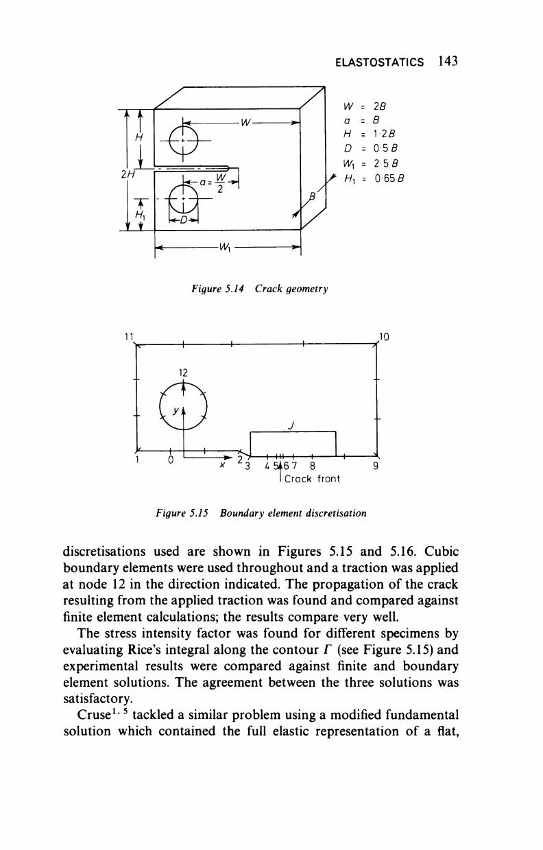
Figure 5.15 Boundary element discretisation
discretisations used are shown in Figures 5.15 and 5.16. Cubic
boundary elements were used throughout and a traction was applied
at node 12 in the direction indicated. The propagation of the crack
resulting from the applied traction was found and compared against
finite element calculations; the results compare very well.
The stress intensity factor was found for different specimens by
evaluating Rice's integral along the contour Γ (see Figure 5.15) and
experimental results were compared against finite and boundary
element solutions. The agreement between the three solutions was
satisfactory.
Cruse
1,5
tackled a similar problem using a modified fundamental
solution which contained the full elastic representation of a flat,
144 ELASTOSTATICS
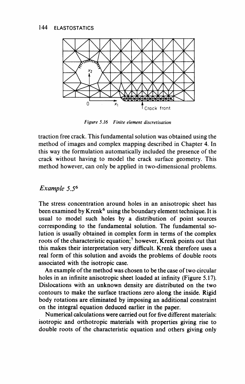
Figure 5.16 Finite element discretisation
traction free crack. This fundamental solution was obtained using the
method of images and complex mapping described in Chapter 4. In
this way the formulation automatically included the presence of the
crack without having to model the crack surface geometry. This
method however, can only be applied in two-dimensional problems.
Example 5.5
6
The stress concentration around holes in an anisotropic sheet has
been examined by Krenk
6
using the boundary element technique. It is
usual to model such holes by a distribution of point sources
corresponding to the fundamental solution. The fundamental so-
lution is usually obtained in complex form in terms of the complex
roots of the characteristic equation;
7
however, Krenk points out that
this makes their interpretation very difficult. Krenk therefore uses a
real form of this solution and avoids the problems of double roots
associated with the isotropic case.
An example of the method was chosen to be the case of two circular
holes in an infinite anisotropic sheet loaded at infinity (Figure 5.17).
Dislocations with an unknown density are distributed on the two
contours to make the surface tractions zero along the inside. Rigid
body rotations are eliminated by imposing an additional constraint
on the integral equation deduced earlier in the paper.
Numerical calculations were carried out for five different materials:
isotropic and orthotropic materials with properties giving rise to
double roots of the characteristic equation and others giving only
ELASTOSTATICS 145
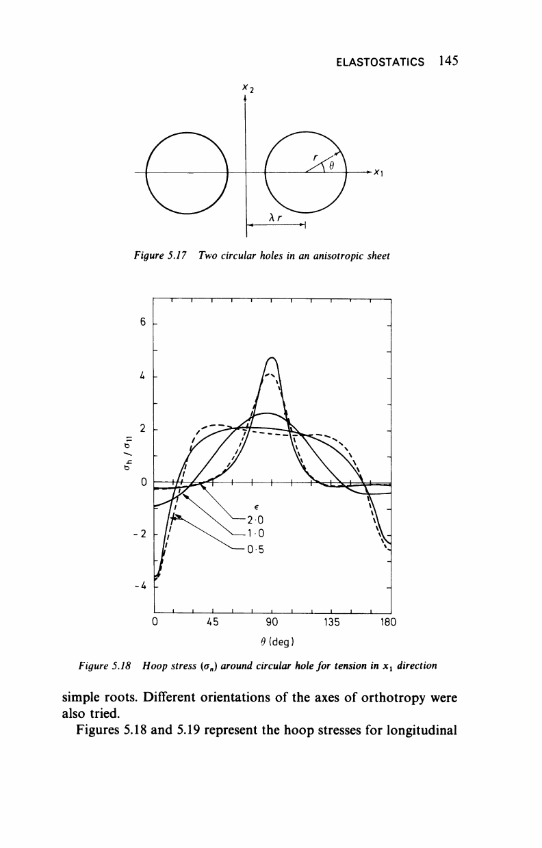
Figure 5.17 Two circular holes in an anisotropic sheet
6 μ
_l I I I L_
0 45 180 90 135
9(6eg)
Figure 5.18 Hoop stress (σ„) around circular
hole
for tension in x
x
direction
simple roots. Different orientations of the axes of orthotropy were
also tried.
Figures 5.18 and 5.19 represent the hoop stresses for longitudinal
..................Content has been hidden....................
You can't read the all page of ebook, please click here login for view all page.