
160 TIME-DEPENDENT AND NON-LINEAR PROBLEMS
exponential series to describe the solution of our problem variable
u(t) accurately. This involves finding a sufficient number of solutions
for differing κ, so that an accurate curve fit to the equation
U(K)
= Σ -^- (6.32)
j=i K-Otj
can be obtained, i.e. to find the constants a, and
Sj
;
(j
ί
= 1, 2, . . ., n).
Having obtained this curve, direct inversion will yield a solution of the
form,
u(t)= X S,e«/ (6.33)
We shall now discuss the application of the Laplace transform
method to the problem of transient elastodynamics.
6.5 TRANSIENT ELASTODYNAMICS
Cruse
1
has solved this problem starting with the field equations based
on the small displacement theory for a linear, isotropic, homo-
geneous, elastic medium (see Chapter 5).
We denote the displacement vector (in two or three dimensions)
associated with each point x in space by,
5(x, t) = (uj(x, t)) (6.34)
Then the equations of motion of the linear, isotropic, elastic body are,
(ci -
c
2
2
)u
L
u
+ c
u
Jm
u
+ bj = d
2
uj/dt
2
(6.35)
where ()j means differentiation with respect to Xy
c
l
is the velocity of dilatational waves where
c?
=
λ
-±^
(6.36)
P
with λ and μ the Lame constants given by,
Ev
V = ^77—, <
6
·
37
)
(l-v)(l-2v)' ^ 2(1+ v)
c
2
is the velocity of distortional waves where,
c = μ/ρ (6.38)
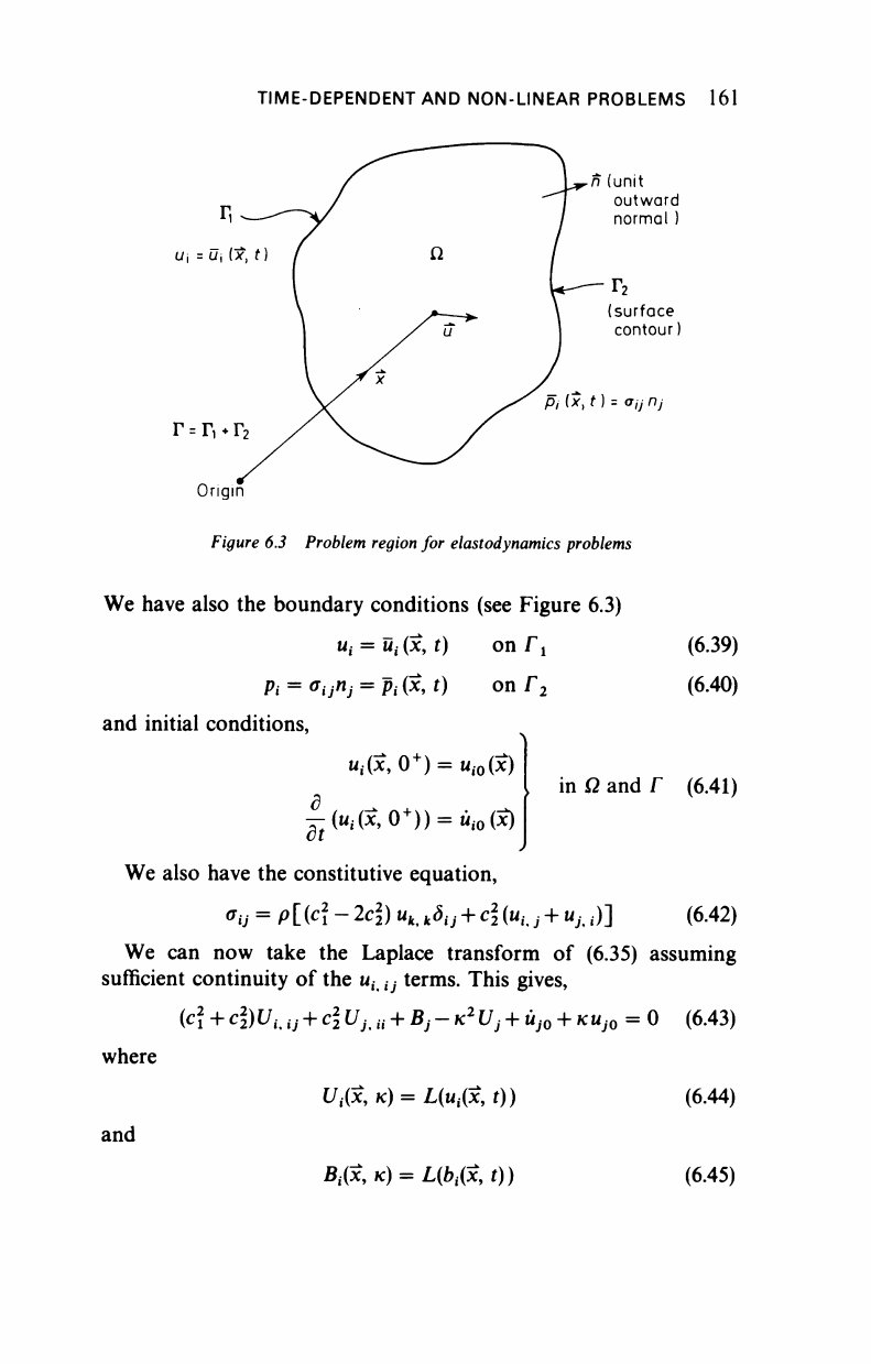
TIME-DEPENDENT AND NON-LINEAR PROBLEMS 161
n (unit
outward
normal )
r
2
(surface
contour)
P/ (*, t)= Gijilj
r
=
r
1
+
r
2
Origin
Figure 6.3 Problem region for elastodynamics problems
We have also the boundary conditions (see Figure 6.3)
u
g
= S,
(x,
t) on Tj
Pi = (fijnj = Pi (*, t) on Γ
2
and initial conditions,
u,(x, 0
+
) =
u
i0
(x)
(6.39)
(6.40)
-(Mx,0
+
)) = ti
iO
(x)
I in Ω and Γ (6.41)
We also have the constitutive equation,
°u = P[(
c
l ~
2c
l)
"*,
k^ij
+ c
(ιι,.,·
+
w,·
,)] (6.42)
We can now take the Laplace transform of (6.35) assuming
sufficient continuity of the u
it (j
terms. This gives,
(c + ci)l/,
l7
+ c U
Jt
u
+
2*,
-
K
2
£/, + u
j0
+ κκ,
0
= 0 (6.43)
where
l/
i
(Jc,ic) = L(ii
j
(x,r)) (6.44)
and
B& κ) = L(bi(x, t)) (6.45)
162 TIME-DEPENDENT AND NON-LINEAR PROBLEMS
The boundary conditions
(6.39)
and (6.40) may also be transformed
in the usual way to give,
Ui(x, κ) = ϋί(χ, κ)
οηΓ
ί
(6.46)
p.(x,
K)
= P,(3c, K) on Γ
2
(6.47)
If we group the body force terms together we can write,
Qj = p(Bj + uj
0
+
KU
J0
)
(6.48)
and hence (6.43) becomes,
(c -
c
2
2
)V
u
u
+ c U
h
a
-
K
2
Uj = - Qj/p (6.49)
Following Doyle
12
and utilising the Galerkin vector we may
deduce the fundamental influence tensors for this equation as,
U
h-^M>-V<0
(6-50)
(a = 2 for two dimensions and a = 4 for three).
For two dimensions φ and χ are given by
*-*·®£[«·®-Ηΐ)]
K
0
, K
x
and K
2
are modified Bessel functions of the third kind of
orders zero, one and two respectively.
13
For three dimensions,
r κτΓ
ί
Kr
J r cfK
2
r
z
κτ) r
(6.52)
3c
2
2
3c
2
e
-
Kr
/
c
i (c\(2>c 3c
t
e
-
Kr
/
c
i
+
—+
1
l-i M^
+
^+l
K
2
r
2
Kr ) r c ] K*r* KY
The fundamental traction tensor components P*
7
may be obtained
using (6.40) and (6.42).
..................Content has been hidden....................
You can't read the all page of ebook, please click here login for view all page.